Macrmolecule Application of Optiprep
OptiPrep™ Application Sheet M01
Preparation of gradient solutions (for macromolecules and macromolecular complexes)
1. OptiPrep™
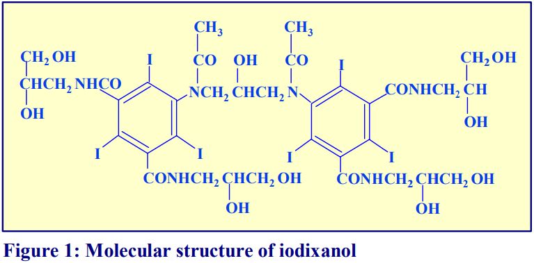
OptiPrep™ is a 60% (w/v) solution of iodixanol in water, density = 1.32 g/ml. Iodixanol is a nonionic molecule with a molecular mass of 1550 (see Figure 1).
2. Handling OptiPrep™
Exposure (several months) of iodixanol solutions to direct sunlight will cause a slow release of iodine (solution turns yellow); OptiPrep™ should therefore be stored away from strong sunlight. On standing, iodixanol may “settle out” of concentrated solutions, which should be well mixed before use.
3. Osmolality
The observed osmolality of OptiPrep™ depends on the mode of measurement (vapour pressure or freezing point); moreover the situation is complicated by the tendency of the iodixanol molecules to associate non-covalently in a concentrated aqueous solution. Thus, measured values of osmolality may be lower than might be expected. Importantly however, when OptiPrep™ is diluted with a buffered isoosmotic solution, the iodixanol oligomers dissociate and all dilutions are isoosmotic. Under normal operating conditions therefore OptiPrep™ behaves as if it had an osmolality of approx 290 mOsm.
4. Preparation of density solutions
Macromolecules and macromolecular complexes cover such a diverse range of particles that it is not possible to give all the possible recipes for the preparation of gradient solutions from OptiPrep™. Instead, the preparation of gradient solutions from two types of general-purpose working solution, based on the use of either NaCl or sucrose as osmotic balancer, are described in this section. Specific examples of gradient solutes for the purification of nucleic acids, proteins, nucleoprotein particles and lipoproteins are briefly discussed in Section 5.
If it is important to maintain the concentration of a particular buffer or additive constant throughout the gradient, then the general strategy is to start by making a dense working solution. For example make a 50% (w/v) iodixanol working solution (WS) by diluting 5 vol. of OptiPrep™ with a 1 vol. of a diluent containing 6x the required concentrations of buffer and additives. The working solution will then contain the correct concentration of additives; this can then be further diluted with the normal medium to provide solutions of lower density. Note that the concentration of any osmotic balancer (e.g. NaCl or sucrose) is not similarly increased six-fold; if it were then the solution would be grossly hyperosmotic. The WS can also be added directly to a sample to adjust its density. Tables 1 and 2 give the density of solutions produced by dilution of a 50% (w/v) iodixanol WS with either 0.85% NaCl, 10 mM Tris-HCl, pH 7.4 (Table 1) or 0.25 M sucrose, 1 mM EDTA, 10 mM Tris-HCl, pH 7.4 (Table 2). In each case the WS contains the same concentration of buffer or buffer + EDTA respectively.
Macromolecules and macromolecular complexes traditionally have been purified in gradients containing high concentrations of sucrose, glycerol, alkali metal salts (e.g. KBr and NaCl) or heavy metal salts (e.g. CsCl). The particles have therefore been isolated in grossly hyperosmotic conditions. OptiPrep™ offers the opportunity to isolate them under more or less isoosmotic conditions. Note therefore that in iodixanol gradients, the macromolecules may have lower densities.

5. Macromolecule-specific buffers
Very often the buffers used in the gradients are specific to the type of macromolecule of macromolecular complex under investigation. Some of the published examples are briefly described in this section.
5a. Nucleic acids
Gradients containing 1 mM EDTA, 10 mM NaCl, 10 mM Tris-HCl, pH 7.5 are not uncommon. See ref 1 for more information of the effect of gradient composition on the banding density of nucleic acids in iodinated density gradient media.
5b. Ribonucleoproteins
Gradients for the study of ribonucleoprotein complexes from both Xenopus and mammalian sources often contain quite high levels of KCl: for example 0.3 M KCl, 2 mM MgCl2 in a 10 or 20 mM HEPES of Tris buffer [2-4], although lower concentrations of 115 mM KCl have also been used [5]. There is nevertheless a wide variety of (often complex) media that are used in gradients for the isolation of ribonucleoproteins and there are several excellent reviews on the fractionation of these complexes in a variety of media [6-8] that give details of the required gradient composition.
5c. DNA-protein complexes
The banding of DNA-protein complexes usually occurs in gradients containing salt since the complexes are unstable in its absence (e.g. 0.14 M NaCl, 1 mM DTT, 0.1 mM EDTA, 10 mM TrisHCl, pH 7.5). Gradients for studying pre-integration complexes; gradients often contain buffered 5 mM MgCl2, 6 mM EDTA, 150 mM KCl with [9] or without DTT [10].
5d. Proteins
Soluble proteins have been banded in gradients produced by dilution of OptiPrep with a simple HEPES-buffered saline, but often other reagents that may stabilize the protein are included. Basi and Rebois [11] for example included 20 mM HEPES-NaOH, pH 8.0, 1 mM EDTA, 1 mM DTT, 2 mM MgSO4 and 0.1% Lubrol PX in iodixanol gradients for studying the sedimentation of proteins. At the concentrations used, these reagents will have little effect on the density or osmolarity of the gradient. Other gradient studies on proteins have used 35 mM PIPES, 0.5 mM MgSO4, 0.1 mM EGTA, 0.5 mM EDTA [12] and 100 mM NaCl, 1 mM EDTA buffered with 50 mM Tris [13].
5e. Lipoproteins
Simple dilutions of OptiPrep with HEPES-buffered saline suffice for the fractionation of lipoproteins and antioxidants may be included at the discretion of the operator.
6. Calculation of density
As long as the density of the diluent is known then Equation 1 can be used to calculate the density of any solution produced from the diluent and a working or stock solution of iodixanol.
Equation 1:
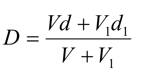
D = density of mixture; V = volume of iodixanol stock solution; d = density iodixanol stock solution;
V1 = volume of diluent; d1 = density of diluent
7. References
1. Ford, T. and Rickwood, D. (1983) Analysis of macromolecules and macromolecular interactions using isopycnic centrifugation In Iodinated density gradient media – a practical approach (ed. Rickwood, D.) IRL Press at Oxford University Press, Oxford, UK. pp 23-42
2. Tafuri, S.R. and Wolffe, A.P. (1993) Selective recruitment of masked maternal mRNA from messenger ribonucleoprotein particles containing FRGY2 (mRNP4) J. Biol. Chem., 268, 24255-24261
3. Han, S-Y., Xie, W., Hammes, S.R. and DeJong, J. (2003) Expression of the germ cell-specific transcription factor ALF in Xenopus oocytes compensates for translational inactivation of the somatic factor TFIIA J. Biol. Chem., 278, 45586-45593
4. Stenina, O.I., Shaneyfelt, K.M. and DiCorleto, P.E. (2001) Thrombin induces the release of the Y-box protein dbpB from mRNA: a mechanism of transcriptional activation Proc. Natl. Acad. Sci. USA, 98, 7277-7282
5. Nielsen, F.C., Nielsen, J., Kristensen, M.A., Koch, G. and Christiansen, J. (2002) Cytoplasmic trafficking of IGF-II mRNA-binding protein by conversed KH domains J. Cell Sci., 115, 2087-2097
6. Houssais, J. F. (1983) Fractionation of ribonucleoproteins from eukaryotes and prokaryotes In Iodinated density gradient media – a practical approach (ed. Rickwood, D.) IRL Press at Oxford University Press, Oxford, UK. pp 43-67
7. Rickwood, D. and Ford, T. C. (1983) Preparation and fractionation of nuclei, nucleoli and deoxyribonucleoproteins In Iodinated density gradient media – a practical approach (ed. Rickwood, D.) IRL Press at Oxford University Press, Oxford, UK. pp 69-89
8. Bommer, U. A., Burkhardt, N. S., Jünemann, R., Spahn, C. M. T., Triana-Alonso, F. J. and Nierhaus, K. H. (1997) Ribosomes and polysomes In Subcellular fractionation – a practical approach (ed. Graham, J. M. and Rickwood, D.) Oxford University Press, Oxford, UK, pp271-301
9. Chen, H. and Engelman, A. (1998) The barrier-to-autointegration protein is a host factor for HIV type 1 integration Proc. Natl. Acad. Sci. USA, 95, 15270-15274
10. Wei, S-Q-. Mizuuchi, K. and Craigie, R. (1997) A large nucleoprotein assembly at the ends of the viral DNA mediates retroviral DNA integration EMBO J., 16, 7511-7520
11. Basi, N. S. and Rebois, R. V. (1997) Rate zonal sedimentation of proteins in one hour or less Anal. Biochem., 251, 103- 109
12. Miller, K.E. and Sheetz, M.P. (2000) Characterization of myosin V binding to brain vesicles J. Biol. Chem., 275, 2598- 2606
13. Hartlieb, B., Muziol., T., Weissenhorn, W. and Becker, S. (2007) Crystal structure of the C-terminal domain of Ebola virus VP30 reveals a role in transcription and nucleocapsid association Proc. Natl. Acad. Sci. USA, 104, 624-629
OptiPrepTM Application Sheet M01; 9th edition, January 2020
OptiPrep™ Application Sheet M02
Preparation of discontinuous and continuous gradients (for macromolecules and macromolecular complexes)
- To access other Application Sheets referred to in the text return to the Macromolecules and Macromolecular Complexes Index; key Ctrl “F” and type the M-Number in the Find Box.
1. Discontinuous gradients
1a Overlayering technique
The most widely used method for producing discontinuous gradients is to start with the densest solution and layer solutions of successively lower densities on top using some form of pipette or syringe. Tilt the centrifuge tube (approx. 45°); place the tip of the pipette or syringe against the wall of the tube, about 1 cm above the meniscus of the denser solution, and gently deliver a slow and steady stream of liquid. This allows the liquid to spread over the tube surface and minimizes any mixing due to a sudden increase in liquid flow. Once a steady flow is established keep the tip of the pipette or syringe just above the meniscus of the liquid and against the wall of the tube.
From a pipette
Use a rubber two- or three-valve pipette filler to aliquot and dispense the gradient solutions. Check that the release valve when pressed gently, allows the delivery of a slow and steady flow of liquid. Do not use a pipette filler that uses positive pressure to deliver the liquid, as a slow even flow is often difficult to attain. Always take up more of the gradient medium than is required as it is easier and more accurate to empty the pipette to a graduation mark than to try to empty it completely.
From an automatic pipette
For small volume gradients an automatic pipette may be used. Always cut off the end of the plastic pipette tip to reduce the flow velocity of the liquid.
From a Pasteur pipette
Plastic Pasteur pipettes can be used conveniently for larger volume gradients, particularly those in calibrated centrifuge tubes. It requires some practise however to maintain a steady liquid flow by depressing the bulb of the pipette.
From a syringe
A syringe with a wide-bore metal filling cannula (i.d. approx 0.8 mm) is suitable for most gradient volumes, but make sure that the barrel can move easily and smoothly when a small pressure is applied. Placing the index finger around the bottom of the plunger, rather than around the barrel, restricts the movement of the plunger when it is depressed and thus achieves a more controlled liquid flow. Always take up more of the gradient medium than is required for the step as it is more accurate to empty the syringe to a graduation mark than to try to empty it completely.
- Metal filling cannulas can be purchased from most surgical instrument suppliers.
1b Underlayering technique
Although the overlayering technique is probably the most widely used, the easier method is to underlayer successively denser solutions beneath the lighter solutions. The only important requirement is that no air bubbles are introduced which may disturb the lower density layers above; for this reason a syringe with a metal filling cannula is the best tool for this procedure. Generally the existing steps are disturbed less as the outflowing liquid spreads upwards through the hemispherical section of
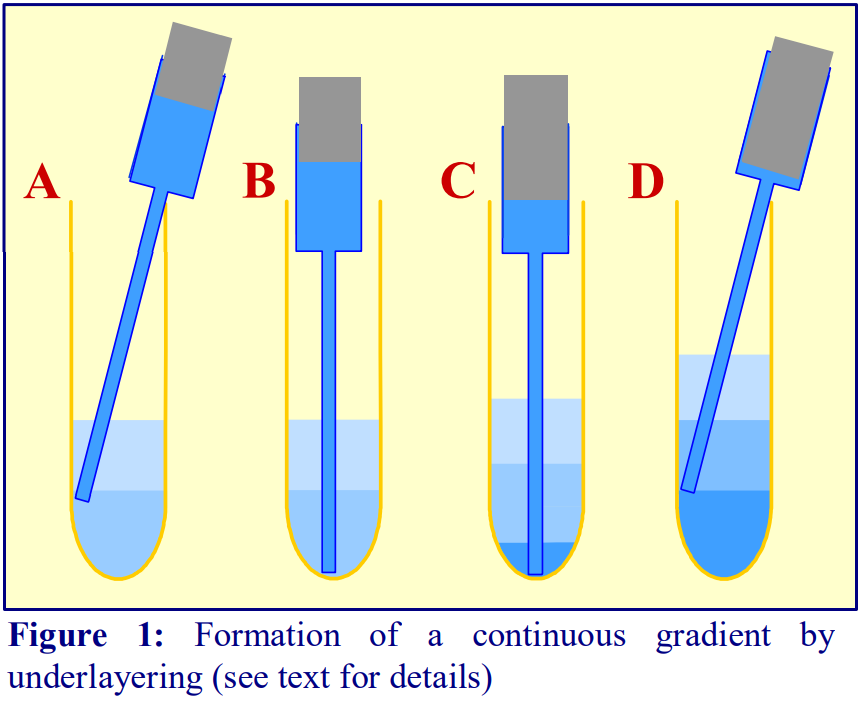
1. To underlayer 4 ml of liquid, take up 5 ml into the syringe and expel to the 4.5 ml mark to ensure that the cannula is full of liquid.
2. Dry the outside of the cannula.
3. Move the tip of the cannula to the bottom of the tube, sliding it slowly down the wall of the tube (Figure 1A-B)
4. Depress the plunger to the 0.5 ml mark (Figure 1C).
5. After a few seconds (to allow all of the liquid to be delivered into the tube) slowly withdraw the cannula, again against the wall of the tube (Figure 1D).
6. Dry the outside of the cannula and repeat the procedure with successively denser solutions.
 2. Continuous gradients
Continuous gradients may be made by allowing discontinuous gradients to diffuse or by using a gradient maker specifically designed for this purpose.
2a By diffusion of discontinuous gradients
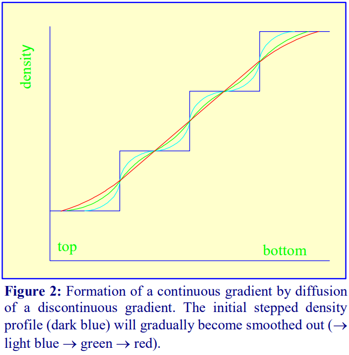
Once a discontinuous gradient is formed, the sharp boundaries between the layers, which are observed as a sudden change in refractive index, start to disappear as the solute molecules diffuse down the concentration gradient from each denser layer to each lighter layer. Thus the density discontinuities between each layer will slowly even out and the gradient will eventually become linear (Figure 2), and given sufficient time the density will become completely uniform.
For a particular medium, the rate of diffusion across an interface is dependent on temperature and the cross-sectional area of the interface. In addition the rate at which the gradient becomes linear will also be a function of the distance between the interfaces. Thus a linear gradient will form more rapidly at room temperature than at 4°C and if the distance between interfaces is reduced and the crosssectional area increased. This can be achieved as follows (refer to Figure 3).
1. Produce a discontinuous gradient by the underlayering (Section 1b) or overlayering (Section1a) method. Unless the gradient is to be very shallow use 3 or 4 layers that increase in steps of about 5-10% (w/v) iodixanol.
2. Seal the tube well with ParafilmⓇ and carefully rotate the tube to a horizontal position and leave for 45-60 min.
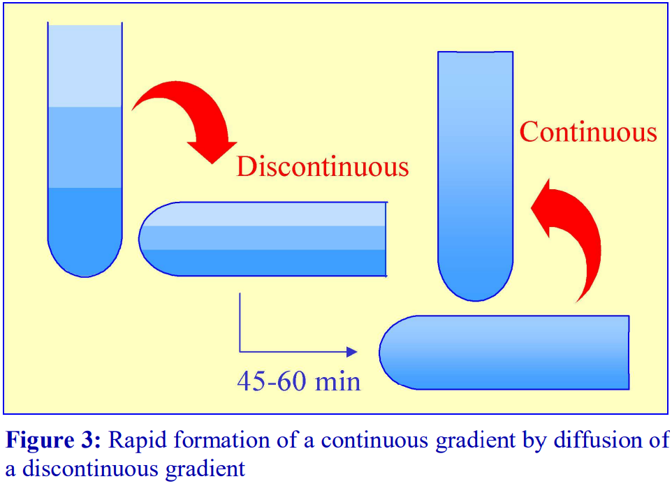 3. Return the tube to the vertical, cool to 4°C if required and apply the sample to the gradient (either over- or underlayered).
The precise timing for the formation of a continuous linear gradient will depend on the dimensions of the tube, the number of layers and the concentrations of iodixanol. A series of trial experiments should be carried out in which the time is varied and the density profile of the formed gradient checked by fractionation and refractive index measurement.
Because the continuous gradient is formed by a physical process, so long as the temperature and time are well controlled, the shape of the gradient is highly reproducible. If the diffusion is allowed to occur in a vertically maintained tube the process will take longer and at 4C it may take more than 10 h. If however the gradients are prepared the day before the experiment and left in the refrigerator overnight this can be a convenient approach. Gradients prepared rapidly at room temperature need to be equilibrated at 4°C prior to loading of the sample. Incorporation of the sample into one or more of the layers eliminates interfaces and can improve resolution, but this useful strategy (used with cells) is unlikely to suit macromolecules or macromolecular complexes that need maintaining at 4C.
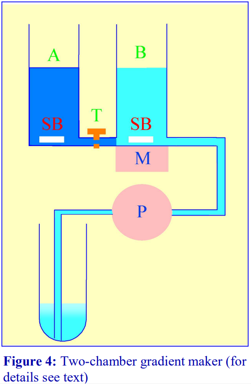 2b Using a two-chamber gradient maker
The traditional way of constructing a continuous gradient is to use a standard two-chamber gradient maker (Figure 4). It
consists of two identical chambers connected close to their bases by a tapped channel (T). One of the chambers (the mixing chamber – B in Figure 4) has an outlet directly opposite the inlet from the tapped channel.
1. Set up the device as shown in Figure 4 with the mixing chamber (B) resting on a magnetic stirrer (M) and the outlet tube leading via a peristaltic pump (P) to the bottom of the centrifuge tube.
2. Place the chosen high-density solution in the non-mixing chamber (A) and then momentarily open the tap (T) to allow dense liquid to fill the connecting tube.
3. Pour an equal volume of the low-density solution in the mixing chamber (B).
4. Place two identical stirring bars (SB) in the two chambers (this ensures that the height of the two solutions is the same).
5. In rapid sequence, switch on the pump (P) and the magnetic stirrer (M) and then open the connecting tap (T). As the levels in the two chambers fall synchronously, reduce the speed of the stirrer to avoid generating air bubbles that may enter the gradient and disturb it.
6. Make sure that the pump is turned off before any air bubbles reach the bottom of the delivery tube at the end of the operation.
- The larger the density difference between the two gradient solutions the more vigorous must be the stirring to ensure good mixing. If the stirring bar in chamber B is too close to the inlet from the connecting tube, it is possible in the initial stages for the low-density medium to back flow into the high-density medium.
- The correct pumping speed depends on the volume of the gradient and the quality of the pump (ideally the outflow from the pump should not pulsate), but for a standard 10-30% (w/v) iodixanol gradient (of 12-15 ml total volume) a flow rate of approx 2 ml/min is satisfactory. Pumps that impart little or no pulsation to the liquid flow are commonly available from many sources.
- The gradient can alternatively be produced high density end-first, in which case the location of the two solutions needs to be reversed and the delivery tube to the centrifuge tube must be placed against the wall of the centrifuge tube near to its top, so the gradient flows down the tube smoothly. This is can pose some problems of mixing in the centrifuge tube if the flow down the tube wall is in the form of large drops rather than a continuous stream (this may be minimized by tilting the tube), on the other hand the tendency of the low density medium to float to the surface of the high density medium in the mixing chamber aids mixing. The Auto Densi-Flow gradient unloader can be used to deposit a gradient high-density end first with no disturbance. Although this device is no longer commercially available, it will be found in many laboratories. For details of this device see Application Sheet M04.
- To guard against air bubbles entering the delivery tube, a bubble trap could be included between mixer and pump. Although air bubbles are a major problem if they reach the bottom of the centrifuge tube (low density first delivery) they are no less a problem for high-density first delivery as they interfere with the smooth flow of liquid down the tube wall.
- It is possible to produce up to three gradients at a time; some gradient mixers have a three-outlet manifold. However such a device requires three tubes to pass through the peristaltic pump. It is the only reliable configuration of the delivery tube; simply splitting the liquid flow from a single tube through the pump cannot guarantee precisely equal delivery to all three tubes.
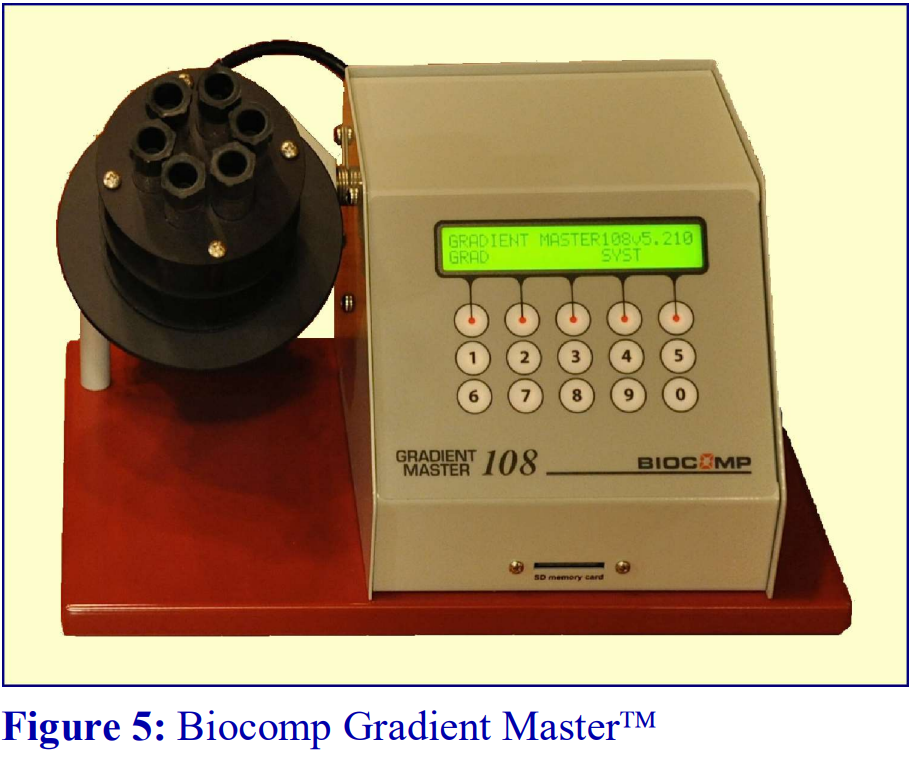 2c Gradient Master™
An alternative device for the generation of continuous density gradients – the Gradient Master™ – produces the gradient by controlled mixing of the low and high-density solutions layered in the centrifuge tube. The tubes are rotated at a pre-set angle (in the drum to the left of the control panel) – usually 80° – to increase the cross-sectional area of the interface – and speed (usually 20 rpm) for about 2 min (Figure 5). The density profile of the gradient generally becomes more shallow with time. The simplicity of the technique and the highly reproducible nature of the gradients make this a very attractive method; up to 6 gradients (17 ml tubes) can be formed at once. Some examples with iodixanol solutions are given in Figures 6 and 7.
- A very important advantage of this technique over the use of a two-chamber gradient mixer is that if it is necessary to make the sample part of the gradient, any potentially hazardous biological sample is contained within the centrifuge tube and does not contaminate the gradient forming device and ancillary tubing.
- For more information on the Gradient Master™ and other similar instruments contact the manufacturers at www.biocompinstruments.com

 2d Freeze-thawing
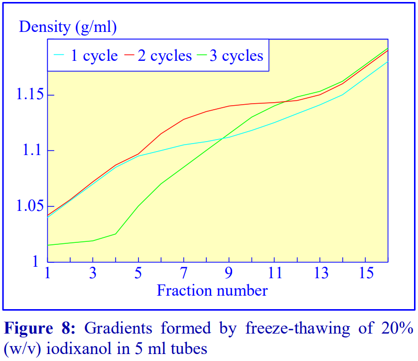
The final manner in which continuous gradients can be produced is by freezing a solution of uniform density for at least 30 min at -20°C and then thawing at room temperature for 30-60 min. These times are for tubes of approximately 5 ml volume. The freeze-thaw cycles can then be repeated; this modulates the density profile of the gradient. Generally as the number of freeze-thaw cycles increases, the gradient becomes markedly less dense at the top. The method can produce gradients that are more or less linear. Because the shape of the gradient depends on the rate of freezing and thawing, as well as the number of freeze-thaw cycles (and the volume of the tube), the precise conditions required need to be worked out for a particular laboratory. Under well-controlled conditions however, the profiles are highly reproducible. An example of the procedure with an iodixanol solution is given in Figure 8 (data kindly supplied by Dr C A Borneque, CNRS, Centre de Génétique Moléculaire, 91198 Gif sur Yvette, France).
2e Non-linear gradients
It is not always desirable to use a linear gradient and either convex, concave, S-shaped or more complex gradient density profiles may be required to effect a particular resolution of particles. Convex gradients are sometimes particularly useful for the resolution of a sample containing a high concentration of particles of a wide range of densities. The steep density profile at the top of the gradient provides stable conditions for high capacity and the shallower high-density region provides high resolution.
From discontinuous gradients by diffusion
If each of the layers of the initially discontinuous gradient is of the same volume then diffusion will produce a linear gradient. The diffusion process however is also a very convenient way of producing a gradient that is not linear with volume. Convex or concave gradients or gradients containing a shallow median section can be produced by increasing the volume of the denser, lighter or median density layers respectively. The shape of the gradient may also be altered by changing the density interval between adjacent layers. Clearly reducing the density interval will make the gradient more shallow. It is important to test the density profile that is formed from such discontinuous gradients, but once satisfactory conditions are established the profile will be highly reproducible.
Using a gradient mixer or Gradient Master
Convex and concave gradients cannot be produced with the standard two-chamber gradient mixer (see Figure 4). However if the non-mixing chamber is made twice the diameter of the mixing chamber, then with low-density solution in the mixing chamber a convex gradient is produced; if the locations of the low density and high-density solutions are reversed, a concave gradient is produced. In a Gradient Master™ (see Section 2c) non-equal volumes of the two density solutions will change gradient shape.
 3. Types of rotor used with preformed gradients
Traditionally, preformed gradients of sucrose or glycerol are run in a swinging-bucket rotor and today this remains the most popular choice of rotor for any density gradient centrifugation. Sedimentation path lengths tend to be long, but because of the relatively low viscosity of iodixanol solutions, centrifugation times need not be excessive. Separation of proteins on the basis of sedimentation velocity in swinging-bucket rotors is commonly carried out overnight. However, because iodixanol is able to form its own gradient by self-generation in the centrifugal field, it is not good practice to carry out buoyant density banding through pre-formed gradients at RCFs in excess of 250,000 gav for more than 3-4 h. Iodixanol molecules towards the bottom of the tube may start to form a selfgenerated gradient and thus deform the pre formed density profile in the high-density region. At lower RCFs (e.g. 100,000 g) there will essentially be no density profile modulation.
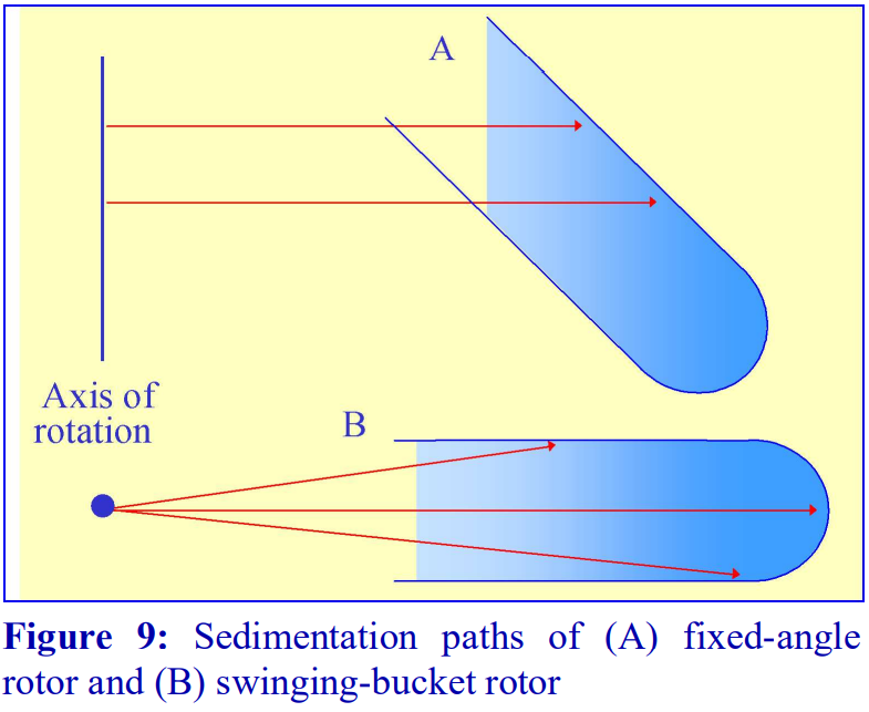
Fixed-angle rotors are generally less frequently used for pre-formed gradients. Because of the angle at which the tube is held, particles tend to sediment to the wall of the tube due to the radial centrifugal field (Figure 9A); this does not occur in a swinging-bucket rotor, although even in this type of rotor, only those particles in the middle of the sample move in a plane parallel to the walls of the tube (Figure 9B). Swinging-bucket rotors were also often perceived as having an advantage over fixed-angle rotors for gradient work since the gradient always maintains the same orientation with respect to the long axis of the tube. However, so long as the particles do not adhere to the wall of the tube, a fixed-angle rotor can provide a useful alternative and there are many successful examples, particularly now that slow acceleration and deceleration facilities are widely available on centrifuges to permit smooth reorientations of the gradient.
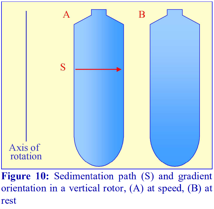 If a fixed-angle rotor is satisfactory for a particular gradient separation, then the shorter sedimentation path length of such a rotor compared to that of a swinging-bucket rotor of the same capacity permits a shorter centrifugation time. This situation is taken to its logical conclusion with a vertical rotor which will have the shortest path length, i.e. the width of the tube and, like the swinging-bucket rotor, the sedimentation or flotation of particles is relatively unaffected by the tube wall (Figure 10). In these rotors therefore, centrifugation times are reduced to a minimum. Analysis of the oligomerization of the ß-amyloid Aß peptide for example needs only 3 h in an iodixanol gradient in a vertical rotor, see Application Sheet M09. In a rotor such as the Beckman VTi65.1 or VTi50 the long axis of the tubes is much larger than their diameter (Figure 10), so the steep gradient formed during centrifugation reorients to a relatively shallow one at rest. Therefore, so long as there is no mixing of the tube contents during deceleration, small volume fractionation of the gradient will provide very high resolution.
- It is important that the gradient is so designed to prevent particles from sedimenting to the wall of the tube, as these will tend to fall back into the medium during reorientation and unloading and thus contaminate the rest of the gradient.
- Near-vertical rotors, which hold the tube at approx. 8° to the vertical, overcome this problem.
- Vertical and near-vertical rotors can provide the most efficient form of centrifugation in gradients. They can be particularly effective for rate-zonal separations, since any sample placed on top of a gradient achieves a very small radial thickness after reorientation.
- Because the surface area of any banded material is much higher in a vertical or near-vertical rotor than in a swinging-bucket rotor during centrifugation, particles that have a significant rate of diffusion (Mr<5×10⁵) may exhibit band broadening due to this diffusion.
The use of large volume zonal rotors for gradient centrifugation is beyond the scope of this text;
for information the reader is referred to relevant review articles [1,2].
4. Types of tube for gradient centrifugation
Choice of tube material (polyallomer, polycarbonate etc) is usually governed by considerations of optical transparency, resistance to chemicals or sterilizing (autoclaving) procedures (see manufacturers specifications for more information); generally speaking there is no specific advantage or disadvantage of using one particular type of tube material for gradient centrifugation from a fractionation point of view. The tube material may also restrict the maximum permitted RCF.
Choice of tube type (open-topped, screw-capped, sealed etc) is dictated by the selection of rotor type, the RCF that is required (many tube types cannot be run at the maximum speed of the rotor); the degree of containment that is required and a consideration of the type of gradient harvesting that is to be carried out. For details on gradient harvesting see Section 4i of Application Sheet M04.
Gradient centrifugation in low-speed and high-speed centrifuges is not generally carried out in special tubes, unless special containment is required; the standard thick walled polycarbonate, polyallomer, polypropylene or polystyrene tubes employed for all low- and high-speed centrifugation are satisfactory.
In ultracentrifugation a wide range of tube styles are available and the reader is directed to the appropriate technical manuals published by the centrifuge companies. Principally polyallomer and polycarbonate or Ultra-Clear™ (Beckman trade-name) are used. For simplicity and convenience only those tubes manufactured by Beckman Instruments will be described although other companies supply an essentially similar range of tubes although there may be some differences in the mode of sealing.
- Swinging-bucket rotors Tubes for swinging bucket rotors are traditionally open topped (the seal being provided the screw-cap on the bucket), thin-walled and made from polyallomer or UltraClear. Occasionally thick-walled polycarbonate is available. See also “Vertical rotors” below.
- Fixed-angle rotors The types of material used for tubes for fixed-angle rotors are broadly similar to those for swinging-bucket rotors. Some of the thick walled tubes are open-topped and do not require caps, others have a variety of capping devices. Thin-walled tubes always require caps. The thick walled variety with a simple screw cap is not ideally suited to some forms of gradient harvesting. For details on gradient harvesting see Section 4i of Application Sheet M04. See also “Vertical rotors”, below.
- Vertical rotors The only types of tube recommended for vertical rotors are thin-walled sealed tubes made either from polyallomer or Ultraclear; these are also available for many swingingbucket and fixed-angle rotors. In swinging-bucket rotors however there is usually a variable reduction in tube volume compared to the standard thin-walled open-topped tubes. Beckman manufacture two types: Quick-Seal™ and Optiseal™, the former are sealed by a heat and the latter by a central plastic plug.
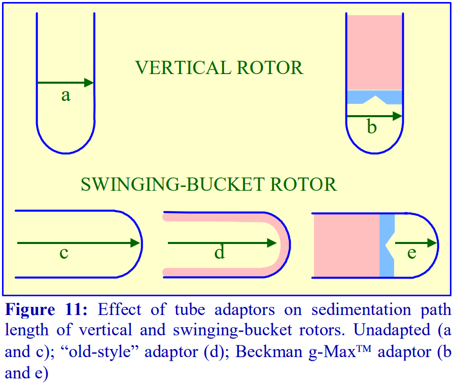 Through the use of adaptors and spacers most rotors accommodate a range of tubes of a volume considerably smaller than that of the rotor tube pocket, many of which may have a restricted maximum RCF (compared to the standard thin walled tube). Traditionally the smaller volume tubes for swinging-bucket and fixed-angle had a much-reduced diameter but the length was only slightly less than that of the fullvolume tube (Figure 11).
- g-Max tubes: Because of the advantage of a short sedimentation path length, some of the swinging-bucket and fixed-angle rotors have been adapted to take shorter sealed tubes so that the path length is reduced. They are also available for vertical rotors but in these rotors the sedimentation path length is unchanged, only the volume is altered (Figure 11).
5. References
1. Graham, J. M. (1978) In Centrifugal separations in molecular and cell biology (ed. G. D. Birnie and D. Rickwood). Butterworths, London, pp 63-85.
2. Graham, J. M. (1992) In Preparative centrifugation – a practical approach (ed. D. Rickwood) IRL Press at Oxford University Press, Oxford, UK, pp 315-350.
OptiPrep™ Application Sheet M02; 8th edition January 2020
OptiPrep™ Application Sheet M03
Self-generated gradients (macromolecules/macromolecular complexes)
1. Background
Iodixanol, like solutions of heavy metal salts (e.g. CsCl), can form a gradient from a solution of uniform density under the influence of the centrifugal field. Once the solute begins to sediment through the solvent a concentration gradient is formed which is opposed by back-diffusion of the solute. With a sufficiently high RCF, at equilibrium, the sedimentation of the solute is exactly balanced by the diffusion and the gradient is stable. It is possible to calculate the time for a selfgenerating gradient to reach equilibrium and it is described by the following equation:
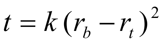
t is the time in hours; rb and rt the distance from the centre of rotation to the bottom and top of the gradient respectively and k is a constant, which depends on the diffusion coefficient and viscosity of the solute and on temperature [1]. The slope of the gradient is given by the equation:
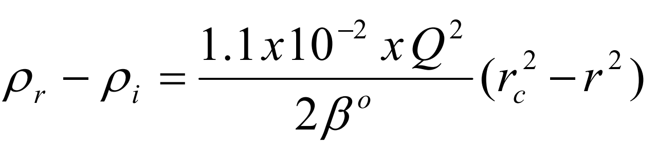
where P r is the density at a point r cm from the axis of rotation, P i is the starting density of the homogeneous solution, rc is the distance in cm from the axis of rotation where the density of the gradient = P i , Q is the rotor speed in rpm and ß o is a constant depending on the solute [1].
The shape of the gradient that is formed for a particular solute thus depends on the following factors:
- sedimentation path length of the rotor
- time of centrifugation
- speed of centrifugation
- temperature
The big advantages of the use of any self-generated gradient are the ease of sample handling (the sample is simply adjusted to the required starting concentration of iodixanol) and the great reproducibility of the gradient density profile under a particular set of centrifugation parameters.
2. Self-generated gradient formation
Iodixanol is able to form useful self-generating gradients in 1-4 h depending on the centrifugation speed and the rotor [2]. Figure 1 compares the gradient density profile generated from 20% (w/v) iodixanol and 20% (w/v) NycodenzⓇ in 0.25 M sucrose in a 20 fixed-angle rotor at 270,000gav for 3 h at 4°C. Clearly a steeper gradient is formed from the iodixanol and this is a function of the higher molecular mass of iodixanol (approx. twice that of NycodenzⓇ): it therefore sediments rather more rapidly and diffuses more slowly.
2a. Types of rotor
Swinging-bucket rotors, which have rather long sedimentation path lengths, are little used for the formation of self-generating gradients. The shorter sedimentation path length rotors are much better suited to this task. Vertical and near-vertical rotors are particularly useful, although some fixed-angle rotors (preferably those with shallow angles of 20-24°) may be used.
Gradients generated in the Beckman TLN100 near-vertical rotor (for the TLX120 table-top ultracentrifuge) which accommodates tubes of 3.5-4.0 ml, the Beckman VTi65.1 vertical rotor (for an appropriate floor-standing ultracentrifuge) which accommodates tubes of approx 11.0 ml (but which can be adapted down to smaller volumes) and the Beckman NVT65 (a near vertical rotor of similar tube capacity to that of the VTi65.1) are particularly useful for iodixanol self-generated gradients. The TLN100 and VTi65.1 rotors have approximately the same sedimentation path length (about 17 mm), that of the NVT65 is marginally longer (approx 25 mm); consequently under the same centrifugation conditions, they generate rather similar gradient profiles.

2b. Time of centrifugation
After 1 h at 15-18oC, centrifugation at approx 350,000gav, gradients generated in the TLN100 are Sshaped (i.e. they contain a relatively shallow region in the middle) and span a relatively narrow density range, while after 3 h, gradients are considerably steeper and cover a much wider density range. Figure 2 compares two starting concentrations of iodixanol at these two times, while Figure 3 compares three times (1, 2 and 3 h) using a 12.5% (w/v) iodixanol starting concentration with the same rotor. The exponential nature of the gradient becomes more apparent with time but times greater than 3 h result in little further change in the shape of the gradient at 350,000g, indicating that an equilibrium point has been reached.
2c. Temperature
Higher temperatures tend to promote the formation of steeper gradients, although this effect is more apparent at shorter times of 1 h than at longer times of centrifugation. Figure 4 compares the formation of gradients at 4C and 18C in the NVT65 rotor at two iodixanol concentrations after centrifugation at approx 340,000gav for 1 h. At 4C, using 0.25 M sucrose as osmotic balancer, the gradients approach equilibrium more slowly: the excellent gradient profiles produced in the VTi65.1 with 15% or 20% (w/v) iodixanol at 4 h are very similar to those at 5 h (Figure 5), compare with Figure 2 (using NaCl as osmotic balancer at 15C).
2d. Iodixanol concentration
Other than changing the density range covered by the gradient (Figures 2 and 4-8) the starting concentration of iodixanol has rather little effect on the rate of gradient formation or shape of gradient profile. The shape of the gradient can be made more linear at lower RCFs by using two layers of iodixanol (e.g. 10% and 30%, w/v) rather than a single uniform concentration (20%, w/v).

2e. RCF
As the RCF decreases, the gradient becomes more shallow in the middle of the tube; the minimum RCF that produces a useful gradient will vary with the time and the rotor type. In the VTi65.1 vertical rotor, even at 170,000gav, a useful shallow gradient is produced within 3 h (Figure 7). In very high performance rotors that can run at up to 150,000 rpm (and also have very short sedimentation path lengths – see next section), self-generated gradients can form in as little as 15 min (Figure 8)

2f. Sedimentation path length
The longer the sedimentation path length of the rotor, the greater the tendency to form S-shaped gradients. Figure 9 compares the gradient formed from 15% or 30% (w/v) iodixanol using the 80Ti fixed-angle rotor with a sedimentation path length of 43 mm (13.5 ml tube volume) at a series of times. At 70,000 rpm, (equivalent to 345,000gav) approx 5 h is required to produce a useful gradient (compare with Figures 2-7).
3. References
1. Dobrota, M. and Hinton, R. (1992) Conditions for density gradient separations In: Preparative centrifugation – a practical approach (ed D. Rickwood) IRL Press at Oxford University Press, Oxford, UK, pp 77-142.
2. Ford, T., Graham, J. and Rickwood, D. (1994) The preparation of subcellular organelles from mouse liver in selfgenerated gradients of iodixanol Anal. Biochem., 220, 360-366.
OptiPrep™Application Sheet M03; 8th edition, January 2020
OptiPrep™ Application Sheet M04
Harvesting gradients
1. Introduction
The mode of harvesting depends very much on the type of tube used for the gradient, the distribution of particles in the gradient and the aim of the fractionation. Thick-walled tubes cannot be unloaded by any of the methods that involve piercing the tube wall with a needle and tubes with a narrow neck, such as some sealed tubes, make access with the tip of an automatic pipette impossible.
2. Tube handling prior to band or gradient recovery
The traditional open topped flexible-walled tubes for swinging-bucket rotors pose few, if any, problems for any mode of sample recovery. Heat-sealed or crimp-sealed tubes pose the biggest problems and for some modes of harvesting it may be necessary to slice off the top, to convert it to an open-topped tube.
- Do not use a scalpel blade
- Use a special tube cutter (Seton Scientific, Los Gatos, CA; sales@setonscientific.com) – the Beckman tube slicer is a possible alternative
3. Recovery of individual bands of material
If the position of the particles of interest has been clearly established and, if there is more than one band in the gradient, the linear separation of those bands is 1 cm, then the band(s) may be removed individually by aspiration.
3a. Using a Pasteur pipette or syringe (applicable to any open-topped tube)
If a syringe is used, attach it to a flat-tipped metal cannula (i.d. 0.8-1.0 mm) not to a syringe needle. Metal filling cannulas may be obtained from any surgical equipment supplies company.
- Place the tip of the pipette or cannula at the top of the band of interest and aspirate the liquid very slowly, moving it across the diameter of the tube.
- To minimise the aspiration of any liquid from below the band, the tip of a glass Pasteur pipette may be fashioned into an L-shape.
- If the band of interest is below other material in the gradient then remove the latter first.
3b. Using a syringe (flexible-walled tubes only)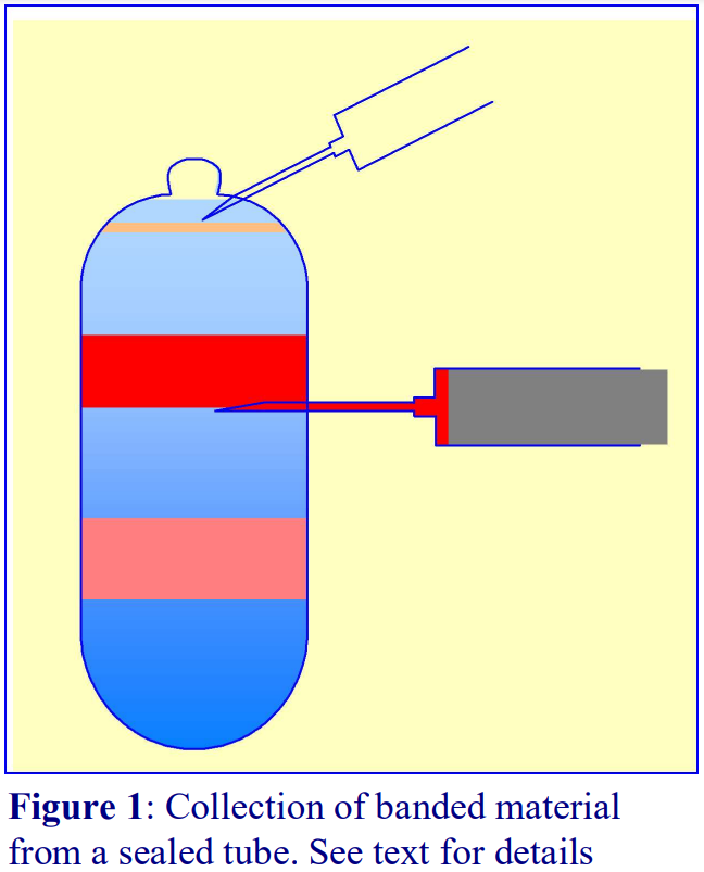
It is also possible to collect a specific band within the gradient by puncturing the tube wall with a needle attached to a syringe.
- To allow easy piercing of the tube wall; the centrifuge tube is best restricted by some sort of tube clamp. Insert the needle just below the band and with the inlet to the needle (bevel uppermost); aspirate the band into the syringe (Figure 1).
- If a sealed tube is used, air must be allowed to displace the falling column of liquid in the tube (see Figure 1) by puncturing the tube close to its top with another syringe needle.
- Once the band has been aspirated, the syringe needle is withdrawn and the hole in the tube sealed with silicone grease.
- The procedure may be repeated to harvest a denser band.
4. Harvesting the entire gradient into a series of equal volume fractions
The volume of each fraction collected from a gradient is determined as much by the operator’s requirements as by the resolving power of the gradient. As a general rule however, the volume of each fraction should be approx 5% of the gradient volume, but this may be decreased or increased for higher or lower resolution respectively.
4a. Using a Pasteur pipette, automatic pipette or syringe (applicable to any open-topped tube)
Most Pasteur pipettes are calibrated on the stem so if the tip of the pipette or cannula (attached to a 1 or 2 ml syringe) is placed at the meniscus, the total gradient may be collected in suitably sized fractions. If an automatic pipette is used, trim the end of the tip to make the orifice diameter 0.8-1.0 mm. The method is however tedious, prone to error and difficult to obtain equal volume fractions because of the need to keep the tip of the cannula or pipette at the meniscus without occasionally
aspirating some air or removing some of the gradient from below the meniscus. For a crude fractionation however into four or five gradient cuts it is quite satisfactory.
4b. Aspiration from the bottom using a peristaltic pump
Ideally the harvesting system should be devised so that the effluent from the tube should not have to pass through a pump, but as long as the dead space volume of the tubing is small compared to the volume of the gradient it is permissible to insert a narrow rigid tube to the bottom of the centrifuge tube and to aspirate the contents (dense-end first). Theoretically, mixing will occur in the vertical section of the collection tubing as the decreasingly dense medium enters the bottom of the tube. In practice however this seems not to be a serious problem, again as long as the enclosed volume of the collecting tube is small compared to that of the gradient.
- If there is a pellet, make sure that the tip of collecting tube is maintained above it.
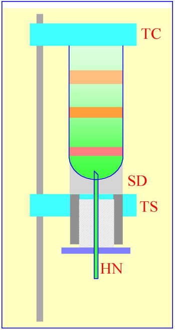 Figure 2: Gradient collection (dense-end first) by tube puncture. The tube is clamped between the sealing disc (SD) and the tube support (TS). A hollow needle (HN) is advanced through the bottom of the tube, sometimes by a screw-device (shown by the hatched area) or, more commonly by a pivoted lever.
4c. Tube puncture
Practically this is best achieved by securing the tube vertically in some form of clamping device and to advance the needle through a rubber seal into the bottom of the tube by a screw or lever mechanism (Figure 2). The Beckman-Coulter Fraction Recovery System incorporates such a device. If sealed tubes are used, then either the central plug should be removed (Optiseal™) or the top punctured with a syringe needle (Quick-Seal™) to allow air to displace the liquid, which exits the tube under gravity. The system is simple and the dead space of the collecting tube is very small and the gradient is collected almost ideally, the hemispherical section of the bottom of the tube directing banded material into the collecting needle. Because of the viscosity of the dense end of some gradients, gravitational flow will be slow at first and then speed up as the viscosity of the liquid decreases. To overcome this, the effluent from the hollow needle can be passed through a small volume peristaltic pump. So long as the dead space of the silicone tubing is small compared to the volume of the gradient, resolution is not seriously sacrificed.
- Thick-walled tubes cannot be used and it may not be a useful method if there is a large pellet, which may obstruct the hollow needle.
- Collecting equal volume fractions by this method or that described in Section 4b is not easy. The low-tech answer is to use calibrated collection tubes, although this requires continual attention from the operator to move on the delivery tube at the appropriate time. This problem is discussed further in Section 4h.

4d. Upward displacement
A dense liquid introduced to the bottom of the tube can displace the entire gradient upwards and with a suitable device attached to the top of the tube, the gradient can be delivered into the collection tubes. The use of a burette to contain the unloading solution does allow the collection of equal volume fractions.
4d-1. Delivery of dense liquid through a central tube inserted into the gradient
A simple device fashioned from a cylindrical block of Perspex (Lucite or acrylic) shown in Figure 3 can be produced by any laboratory workshop. To fit flexible-walled tubes the cylinder should be slightly tapered towards the bottom (not shown in figure). The block contains a central channel, which leads to a hollowed-out cone, and a side-arm, which connects with the central channel. The dense unloading solution is introduced to the bottom via a long metal cannula inserted down the central channel and through the gradient (Figure 4). The gradient is displaced upwards by the incoming dense liquid into the cone and an O-ring around the cannula diverts the flow into the collection tubes via the side-arm.
For rigid-walled open-topped tubes the collecting device requires sealing on to the tube with a gasket, under pressure. Such a device can indeed be used for any type of tube and one is incorporated as one of the options in the Beckman-Coulter Fraction Recovery System.
By placing the dense unloading solution in a burette and delivering it to the bottom of the centrifuge tube via a peristaltic pump (Figure 4), the unloading process can be executed at a uniform flow rate
By using the graduations on the burette to signal the manual advancement of the delivery tube to the next collection tube, it is the only method that guarantees equal volume fractions.
The gradient could alternatively be collected using an automated fraction collector (see Sections 4g and 4h).
The best unloading medium is a low viscosity, dense, non-water-miscible, fluorocarbon such as perfluorodecalin (P = 1.9 g/ml). This was previously commercially available from Axis-Shield and its distributors as Maxidens™. Perfluorodecalin can currently be purchased from F2 Chemicals Ltd, Lea Lane, Lea Town, Preston PR4 0RZ, UK (tel: +44 (0)1772 775802, fax +44 (0)1772 775808). Also available from the same company is a similar fluorocarbon containing a blue dye (Flutec-blue), which makes visual assessment of the progress of gradient unloading very easy.
The rate of gradient unloading should be 1-2 ml/min for 10-20 ml gradients and 0.5-1.0 ml/min for smaller volume gradients.
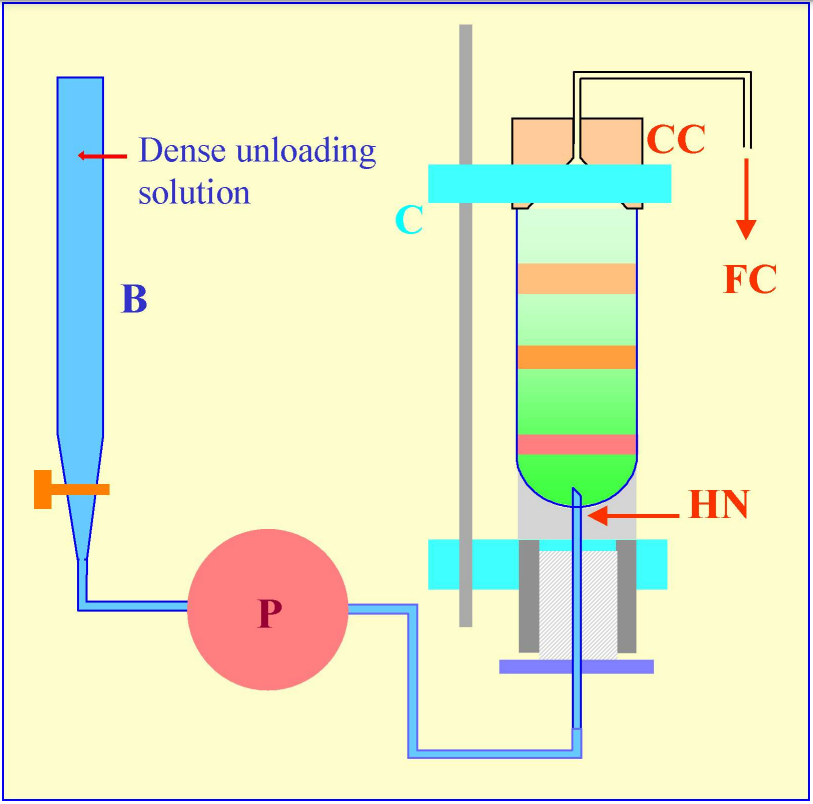 Figure 5: Gradient harvesting by upward displacement with a dense medium delivered by tube puncture. The hollow needle (HN) is completely filled with the dense unloading solution from the burette (B) using the peristaltic pump (P) before the tube is located within the clamping device of a Beckman-Coulter Fraction Recovery System. The conical collection head (CC) is located sealed on to the tube, and the tube held vertically, by the clamp (C). When the pump (P) is reactivated after puncturing the tube, the dense unloading solution displaces the gradient upwards through the conical collection head (CC) and into the fraction collection tubes (FC).
4d-2. Delivery of dense liquid by tube puncture
An alternative mode of delivering the dense unloading solution to the bottom of the tube is by tube puncture. In this case the burette is attached via the pump to the lower end of the hollow needle (Figure 5), which must be primed with the dense solution, prior to tube puncture. The hollow needle (HN) of the Beckman-Coulter Fraction Recovery System has an important design feature – the exit port is on the vertical side of the needle, thus its sharp point is solid. This not only facilitates tube puncture, fragments of tube material removed by the puncturing process or any pellet in the tube, are much less likely to impede the flow of the dense unloading solution than if the exit port was tip-located, as in a standard syringe needle.

4e. Automatic aspiration from the meniscus
The Auto Densi-Flow™, produced by the Labconco Corporation comprises a hollow metal tube that terminates in a small collection head (Figures 6 and 7); the upper end of the tube is connected to a peristaltic pump, which aspirates the gradient. The motor, which is activated when the electronic probe (mounted at the side of the collection head) is in a non-conductive medium (air), advances the collection head towards the gradient until the tip of the probe reaches the meniscus of the gradient (Figure 7, 1 and 2). Now the tip of the probe is in an aqueous conductive medium, the motor stops and the gradient starts to be aspirated by the pump and the meniscus falls (Figure 7, 3). The motor is consequently re-activated as the meniscus recedes from the probe and the collection head advances further downwards until again the probe reaches the meniscus (Figure 7,4) and so on. For clarity, the procedure has been described and shown in Figure 7 in an exaggerated step-like manner. In reality, the aspiration of the gradient and the steady advance of the collection head occur almost simultaneously. In this way the entire gradient is collected in a smooth and continuous fashion.
- Note that the collection head of this device also provides an excellent means of depositing a continuous gradient, dense end first, from a two-chamber gradient maker. In this mode the motor moves the collection head upwards; the sequential activation and deactivation of the motor by the rising meniscus being the reverse of the collection mode.
- IMPORTANT NOTE: although this device is no longer produced by Labconco, many remain available in laboratories and second hand machines are available from instrument “recycling” companies on the internet.
4f. Biocomp Instruments piston fractionator
Rather different to the other types of fractionator, the Biocomp piston fractionator comprises a piston containing a central channel, which at its lower end expands outwards in the form of a curved conical section. As the piston advances down the tube, the gradient is displaced upwards into the central channel. The progressively decreasing volume of the conical section experienced by the displaced liquid effectively increases the linear separation of particles in the gradient and so maximises resolution. The device is available in conjunction with a detection system (and the Biocomp Gradient Master gradient former – see Application Sheet M02 Section 2c). The device is only suitable for open-topped tubes and tubes of different diameters require their own piston.
4g. Integrated automatic gradient harvesting process
In the system illustrated in Figure 8, the Labconco Auto Densi-flow gradient unloader is being used to harvest the gradient (from the meniscus) from a standard tube for a swinging-bucket rotor. The effluent from the peristaltic pump on top of the Auto Densi-flow is directed to the collection head of a Gilson FC205 fraction collector for dispensing into a 96-well polypropylene “MasterBlock DeepWell” plate (Greiner Bio-One Inc). These MasterBlocks can easily accommodate volumes of up to 2.0 ml. The multi-well plate format for gradient collection allows simple gradient analysis if the gradient fractions are subsequently sampled using a multiple channel automatic pipette (see below); it also provides an easy means of storage. A standard 96-well plate can replace the large-volume MasterBlock for the collection of smaller gradient volumes.
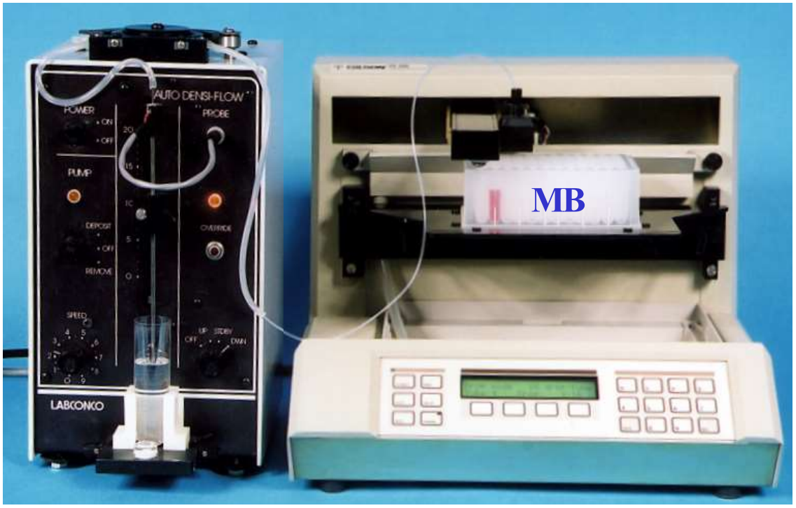 Any gradient unloader that incorporates a peristaltic pump to maintain a reasonably consistent flow rate can be linked up to fraction collector, but note that as the density of the liquid progressively changes so do other physical parameters such as viscosity and surface tension. Drop size will thus vary during the collection process and fraction volumes will change progressively during a drop-counting collection process. So whether the fraction advance is signaled by drop number or time, there will be a progressive change in fraction volume whose severity depends on the density-range of the gradient. Nevertheless if this change is acceptable, it will at least be reproducible from gradient to gradient. This fraction collection system has been used very successfully for analysis of lipoprotein banding in self-generated iodixanol gradients [1,2].
4h. Influence of tube type on harvesting strategy
- Open topped thin walled tubes (polyallomer, polycarbonate or Beckman Ultraclear™) for swinging-bucket or fixed-angle rotors can be unloaded by any of the above methods.
- Thick-walled open-top tubes can be unloaded by any of the methods except tube puncture (Sections 4c and 4d-2).
- Thick-walled tubes (screw-capped) with a wide shoulder are best unloaded from the meniscus (Section 4e) using the Labconco Auto Densi-flow™ or aspiration from the bottom (Section 4b). Upward displacement (Section 4d-1) may be satisfactory if the shoulder is narrow, sloped or rounded, otherwise material may get trapped at the shoulder.
- Heat-sealed or crimp-sealed tubes cannot be unloaded directly by any of the methods except tube puncture (Section 4c). Any other method of unloading requires the tube to be cut horizontally just below the shoulder (see Section 2). This is might cause disturbance to the gradient unless carried out very carefully.
- Sealed tubes that are sealed by a central plastic plug (e.g. Beckman Optiseal™ tubes) can be unloaded by any of the methods. Note however that upward displacement is best carried out using the Section 4d-2 option with a length of Teflon tubing secured to the neck of the tube by a silicone rubber collar to carry the gradient effluent to the collection tubes. Note also that the neck of some of the smaller volume sealed tubes may be too narrow to accept the collection head of the Labconco Auto Densi-flow machine (Section 4e).
5. References
1. Graham, J., Higgins, J. A., Gillott, T., Taylor, T., Wilkinson, J., Ford, T. and Billington, D. (1996) A novel method for the rapid separation of plasma lipoproteins using self-generated gradients of iodixanol Atherosclerosis, 124, 125-135
2. Sawle, A., Higgins, M.K., Olivant, M.P. and Higgins, J.A. (2002) A rapid single-step centrifugation method for determination of HDL, LDL, and VLDL cholesterol, and TG, and identification of predominant LDL subclass J. Lipid Res., 43, 335-343
OptiPrep™ Application Sheet M04; 7th edition, January 2020
OptiPrep™ Application Sheet M05
Analysis of gradients
- To access other Application Sheets referred to in the text: return to the 2020Macroapp file and select the appropriate M-number.
1. Density determination
Once gradients have been fractionated, it is often important that the density of each fraction is measured accurately. The most direct method is to weigh accurately known volumes of liquid using a pycnometer; however, this is very time consuming and it is more convenient to determine the density of a fraction by measuring the refractive index, which has the added advantage of requiring as little as 20-50 µl of sample. The simple linear relationship between refractive index () and the density () is = A – B. The refractive index of gradient solutions is increased by the presence of other solutes (e.g. sucrose and NaCl), thus the values of the two constants A and B vary with the presence and concentration of the solute.
For extensive tables relating % (w/v) concentration of iodixanol, density and refractive index of solutions used for the macromolecular analysis see Application Sheet M01
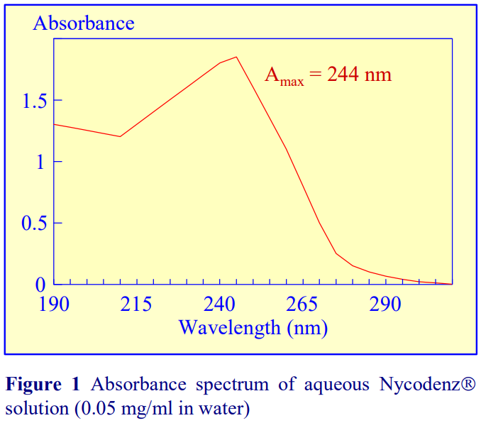 If a refractometer is not available then an alternative method of determining the density of gradient fractions is to measure the absorbance (optical density) of the fractions. All iodinated density gradient media absorb strongly in the UV (see Figure 1). If the absorbance is measured at approx 244 nm (the absorbance maximum for Nycodenz and iodixanol) the gradient samples will need to be diluted 1:10,000 with water to get an absorbance value that can be measured accurately. Table 1 gives a few values for iodixanol solutions, measured in a standard 1 cm path length quartz cell in a single beam spectrophotometer. The need to dilute the solution also means that any other potentially interfering material will be diluted out at the same time.
Alternatively, if the absorbance is measured at a higher wavelength, dilution is not required. Table 2 gives a few absorbance values for Nycodenz solutions at 350 nm and 360 nm. Care must be taken to use the correct blank to ensure that other components in the gradient fractions that absorb at, or near these wavelengths do not interfere with the measurement of the gradient medium.
1a Absorbance measurements using a Multi-well Plate Reader
The wide availability of Multi-well Plate Readers which routinely have the facility for measurement of absorbance at 340 nm considerably simplify the measurement of absorbance on gradient fractions, particularly if the gradient has already been collected in a multi-well plate. Multiple-channel automatic pipettes also facilitate the transfer of liquid aliquots between plates.
1. Transfer 100 l of each of the fractions into 100 l of water in the wells of a second plate.
2. Complete the transfer and mixing by three repeated aspirations into and expulsions from the pipette tips.
3. Measure the absorbance of the solutions in each well in a standard plate reader using a 340 nm filter, against a suitable blank.
For iodixanol concentrations above 35% (w/v), it may be necessary to make a second dilution of the solutions (again 100 l into 100 l of water) to avoid absorbance values above 1.2.
Six different types of multi-well plate have been tested for their suitability. A flat-bottomed 96- well polystyrene plate, which has the lowest background absorbance of any plate tested (approx 0.130 at 340 nm), is available from Greiner BioOne Inc (Cat. # 655101). The inter-well variability of the absorbance was also one of the lowest of all those tested ( 0.007).
Absorbance values of a range of iodixanol solutions produce by dilution of OptiPrep with either saline or 0.25 M sucrose are given in Tables 3 and 4 respectively. The absorbance measurements were made against saline and 0.25 M sucrose blanks, which accounts for the slight distortion of the measured values of samples diluted with sucrose.
2. Particle detection
Although the quantitative distribution of cells through a gradient can be determined by using a haemocytometer or an electronic particle counter, turbidometric analysis is a more general method used for all types of light-scattering particles. Particulate matter can be detected and semi-quantified by light-scattering measurements at 500-600 nm, while particles containing macromolecules bearing porphyrin prosthetic groups (e.g. haem groups) can be monitored by Soret band absorbance at 400- 420 nm.
3. Nucleic acids, proteins and polysaccharides
Although solutions of iodinated media absorb strongly in the ultraviolet region of the spectrum, as their absorbance maximum is different to that of proteins and nucleic acids, it may be possible in some cases, through use of the correct blank (i.e. from a blank gradient unloaded in exactly the same manner as the test gradient) to determine their distribution spectrophotometrically. Normally however, nucleic acids, proteins and polysaccharides are assayed spectrophotometrically by chemical methods (Table 5 and ref 2). Unlike metrizamide, neither Nycodenz nor iodixanol contain a sugar residue, therefore they do not interfere with the orcinol or diphenylamine reactions for the estimation of the ribose and deoxyribose of RNA and DNA respectively [3]; polysaccharides and sugars can be determined using the phenol/H2SO4 assay [4]. Sensitive dye binding assays for protein [5,6] and DNA [7] are also unaffected by the presence of the gradient media. Protein assays based on Coomassie blue give the most reliable data. The Folin Ciocalteu reagent [8] however cannot be carried out unless the concentration of Nycodenz or iodixanol is less than 5% (w/v): this situation however can often be attained if the final assay volume is 1-2 ml and the volume of gradient fraction used is 50 µl. Even at higher concentrations of gradient medium, an appropriate correction can be made to produce a linear relationship between protein concentration and absorbance (Table 6 gives an example). In addition to these spectrophotometric methods, fluorimetric assays of nucleic acids [9,10] and proteins [11] can also be carried out in the presence of Nycodenz or iodixanol. Many of these protocols are listed in ref 12.
4. Radioactivity assays
Analysis of gradients material may either involve the radiolabeling of the material prior to fractionation or the use of radiolabeled reagents in functional assays. Nycodenz and iodixanol quench 3H, 32P and 14C to an extent that is dependent on the energy of the emission, although, as shown in Figure 2, the degree of quenching is also dependent upon the scintillant used. Toluene-based scintillant, containing 4.0 g 2,5-diphenyloxazole (PPO) and 0.05 g 1.4-bis – 2(5-phenyloxazolyl) benzene, (POPOP) per litre and mixed with one half its volume of Triton X-100 is quite resistant to quenching, while Brays scintillant is much less suitable. The extent of quenching may be minimized by diluting the samples prior to counting, or it can be eliminated completely by acid precipitating the material in the gradient fractions and counting each precipitate after collection on filters and drying.
5. Electrophoresis
SDS-polyacrylamide and agarose gel electrophoresis can be carried out directly on gradient samples, as long as the concentration of protein or nucleic acid in the gradient fractions is sufficiently high for analysis. If the protein for example requires concentration, neither Nycodenz nor iodixanol interfere with TCA precipitation.
6. Removal of gradient medium and concentration of fractions
It may be necessary to remove either Nycodenz or iodixanol from the gradient fractions either to concentrate the banded material or if the medium does interfere with some add-on process.
Removal of iodixanol and Nycodenz from gradient samples containing macromolecules and macromolecular complexes is best achieved by filtration through microcentrifuge ultrafiltration cones such as those manufactured by Whatman (Vectaspin) or Millipore (Amicon Ultra 4). Successful use of two other membrane devices has been reported in the literature – Vivaspin membranes from Sartorius and Centricon Plus 70 centrifugal filters from Millipore, or a PBHK Centrifugal Plus-20 filter unit with an Ultracel PL membrane. An alternative is dialysis in large-pore size tubing or in a GeBAflex dialysis tube (Gene Bio Applications (GeBA) Ltd.). The latter are certainly more convenient than dialysis tubing for small volumes, the tubes are available with 0.25, 0.8 and 3.0 ml capacities and MWt cut-offs up to 14,000. Passage down a column of Sephadex G25 is another possibility.
7. References
1. Schroeder, M., Schafer, R. and Friedl, P. (1997) Spectrophotometric determination of iodixanol in subcellular fractions of mammalian cells Anal. Biochem., 244, 174-176
2. Rickwood, D., Ford, T. and Graham, J. (1982) Nycodenz: A new nonionic iodinated gradient medium Anal. Biochem., 123, 23-31
3. Schneider, W.C. (1957) Determination of nucleic acids in tissues by pentose analysis Meth. Enzymol., 3, 680-684
4. Dubois, M., Gilles, K.A., Hamilton, J.K., Rebers, P.E. and Smith, F. (1956) Colorimetric method for determination of sugars and related substances Anal. Chem., 28, 350-356
5. Schaffner, W. and Weissman, C. (1973) A rapid, sensitive, and specific method for the determination of protein in dilute solution Anal. Biochem., 56, 502-510
6. Bradford, M. (1976) A rapid and sensitive method for the quantitation of microgram quantities of protein utilizing the principle of protein-dye binding Anal. Biochem., 72, 248-254
7. Peters, D.L. and Dahmus, M.E. (1979) A method of DNA quantitation for localization of DNA in metrizamide gradients Anal. Biochem., 93, 306-311
8. Lowry, O.H., Rosebrough, N.J., Farr, A.L. and Randall, R.J. (1951) Protein measurement with the Folin phenol reagent J. Biol. Chem., 193, 265-275
9. Fong, J., Schaffer, F.L. and Kirk, P.K. (1953) The ultramicrodetermination of glycogen in liver. A comparison of the anthrone and reducing-sugar methods Arch. Biochem. Biophys., 45, 319-326
10. Karsten, U. and Wollenberger, A. (1977) Improvements in the ethidium bromide method for direct fluorometric estimation of DNA and RNA in cell and tissue homogenates Anal. Biochem., 77, 464-469
11. Bohlen, P., Stein, S., Dairman, W. and Udenfriend, S. (1973) Fluorometric assay of proteins in the nanogram range Arch. Biochem. Biophys., 155, 213-220
12. Ford, T. and Graham, J.M. (1983) Enzymatic and chemical assays compatible with iodinated density gradient media In: Iodinated Density Gradient Media – a practical approach (ed D. Rickwood) IRL Press at Oxford University Press, Oxford, UK, pp 195-216
OptiPrepTM Application Sheet M05; 6th edition, January 2020
OptiPrep™ Application Sheet M05
Analysis of gradients
- To access other Application Sheets referred to in the text: return to the 2020Macroapp file and select the appropriate M-number.
1. Density determination
Once gradients have been fractionated, it is often important that the density of each fraction is measured accurately. The most direct method is to weigh accurately known volumes of liquid using a pycnometer; however, this is very time consuming and it is more convenient to determine the density of a fraction by measuring the refractive index, which has the added advantage of requiring as little as 20-50 µl of sample. The simple linear relationship between refractive index () and the density () is = A – B. The refractive index of gradient solutions is increased by the presence of other solutes (e.g. sucrose and NaCl), thus the values of the two constants A and B vary with the presence and concentration of the solute.
For extensive tables relating % (w/v) concentration of iodixanol, density and refractive index of solutions used for the macromolecular analysis see Application Sheet M01
If a refractometer is not available then an alternative method of determining the density of gradient fractions is to measure the absorbance (optical density) of the fractions. All iodinated density gradient media absorb strongly in the UV (see Figure 1). If the absorbance is measured at approx 244 nm (the absorbance maximum for Nycodenz and iodixanol) the gradient samples will need to be diluted 1:10,000 with water to get an absorbance value that can be measured accurately. Table 1 gives a few values for iodixanol solutions, measured in a standard 1 cm path length quartz cell in a single beam spectrophotometer. The need to dilute the solution also means that any other potentially interfering material will be diluted out at the same time.
Alternatively, if the absorbance is measured at a higher wavelength, dilution is not required. Table 2 gives a few absorbance values for Nycodenz solutions at 350 nm and 360 nm. Care must be taken to use the correct blank to ensure that other components in the gradient fractions that absorb at, or near these wavelengths do not interfere with the measurement of the gradient medium.


1a Absorbance measurements using a Multi-well Plate Reader
The wide availability of Multi-well Plate Readers which routinely have the facility for measurement of absorbance at 340 nm considerably simplify the measurement of absorbance on gradient fractions, particularly if the gradient has already been collected in a multi-well plate. Multiple-channel automatic pipettes also facilitate the transfer of liquid aliquots between plates.
1. Transfer 100 ul of each of the fractions into 100 ul of water in the wells of a second plate.
2. Complete the transfer and mixing by three repeated aspirations into and expulsions from the pipette tips.
3. Measure the absorbance of the solutions in each well in a standard plate reader using a 340 nm filter, against a suitable blank.
For iodixanol concentrations above 35% (w/v), it may be necessary to make a second dilution of the solutions (again 100 l into 100 l of water) to avoid absorbance values above 1.2.
Six different types of multi-well plate have been tested for their suitability. A flat-bottomed 96- well polystyrene plate, which has the lowest background absorbance of any plate tested (approx 0.130 at 340 nm), is available from Greiner BioOne Inc (Cat. # 655101). The inter-well variability of the absorbance was also one of the lowest of all those tested (± 0.007).
Absorbance values of a range of iodixanol solutions produce by dilution of OptiPrep™ with either saline or 0.25 M sucrose are given in Tables 3 and 4 respectively. The absorbance measurements were made against saline and 0.25 M sucrose blanks, which accounts for the slight distortion of the measured values of samples diluted with sucrose.


2. Particle detection
Although the quantitative distribution of cells through a gradient can be determined by using a haemocytometer or an electronic particle counter, turbidometric analysis is a more general method used for all types of light-scattering particles. Particulate matter can be detected and semi-quantified by light-scattering measurements at 500-600 nm, while particles containing macromolecules bearing porphyrin prosthetic groups (e.g. haem groups) can be monitored by Soret band absorbance at 400- 420 nm.
3. Nucleic acids, proteins and polysaccharides
Although solutions of iodinated media absorb strongly in the ultraviolet region of the spectrum, as their absorbance maximum is different to that of proteins and nucleic acids, it may be possible in some cases, through use of the correct blank (i.e. from a blank gradient unloaded in exactly the same manner as the test gradient) to determine their distribution spectrophotometrically. Normally however, nucleic acids, proteins and polysaccharides are assayed spectrophotometrically by chemical methods (Table 5 and ref 2). Unlike metrizamide, neither NycodenzⓇ nor iodixanol contain a sugar residue, therefore they do not interfere with the orcinol or diphenylamine reactions for the estimation of the ribose and deoxyribose of RNA and DNA respectively [3]; polysaccharides and sugars can be determined using the phenol/H2SO4 assay [4]. Sensitive dye binding assays for protein [5,6] and DNA [7] are also unaffected by the presence of the gradient media. Protein assays based on Coomassie blue give the most reliable data. The Folin Ciocalteu reagent [8] however cannot be carried out unless the concentration of NycodenzⓇ or iodixanol is less than 5% (w/v): this situation however can often be attained if the final assay volume is 1-2 ml and the volume of gradient fraction used is 50 µl. Even at higher concentrations of gradient medium, an appropriate correction can be made to produce a linear relationship between protein concentration and absorbance (Table 6 gives an example). In addition to these spectrophotometric methods, fluorimetric assays of nucleic acids [9,10] and proteins [11] can also be carried out in the presence of NycodenzⓇ or iodixanol. Many of these protocols are listed in ref 12.


4. Radioactivity assays
Analysis of gradients material may either involve the radiolabeling of the material prior to fractionation or the use of radiolabeled reagents in functional assays. NycodenzⓇ) and iodixanol quench 3H, 32P and 14C to an extent that is dependent on the energy of the emission, although, as shown in Figure 2, the degree of quenching is also dependent upon the scintillant used. Toluene-based scintillant, containing 4.0 g 2,5-diphenyloxazole (PPO) and 0.05 g 1.4-bis – 2(5-phenyloxazolyl) benzene, (POPOP) per litre and mixed with one half its volume of Triton X-100 is quite resistant to quenching, while Brays scintillant is much less suitable. The extent of quenching may be minimized by diluting the samples prior to counting, or it can be eliminated completely by acid precipitating the material in the gradient fractions and counting each precipitate after collection on filters and drying.
5. Electrophoresis
SDS-polyacrylamide and agarose gel electrophoresis can be carried out directly on gradient samples, as long as the concentration of protein or nucleic acid in the gradient fractions is sufficiently high for analysis. If the protein for example requires concentration, neither NycodenzⓇ) nor iodixanol interfere with TCA precipitation.
6. Removal of gradient medium and concentration of fractions
It may be necessary to remove either NycodenzⓇ or iodixanol from the gradient fractions either to concentrate the banded material or if the medium does interfere with some add-on process. Removal of iodixanol and NycodenzⓇ from gradient samples containing macromolecules and macromolecular complexes is best achieved by filtration through microcentrifuge ultrafiltration cones such as those manufactured by Whatman (VectaspinⓇ) or Millipore (AmiconⓇ Ultra 4). Successful use of two other membrane devices has been reported in the literature – Vivaspin membranes from Sartorius and Centricon Plus 70 centrifugal filters from Millipore, or a PBHK Centrifugal Plus-20 filter unit with an Ultracel PL membrane. An alternative is dialysis in large-pore size tubing or in a GeBAflex dialysis tube (Gene Bio Applications (GeBA) Ltd.). The latter are certainly more convenient than dialysis tubing for small volumes, the tubes are available with 0.25, 0.8 and 3.0 mlcapacities and MWt cut offs up to 14,000. Passage down a column of Sephadex G25 is another possibility.
7. References
1. Schroeder, M., Schafer, R. and Friedl, P. (1997) Spectrophotometric determination of iodixanol in subcellular fractions of mammalian cells Anal. Biochem., 244, 174-176
2. Rickwood, D., Ford, T. and Graham, J. (1982) Nycodenz: A new nonionic iodinated gradient medium Anal. Biochem., 123, 23-31
3. Schneider, W.C. (1957) Determination of nucleic acids in tissues by pentose analysis Meth. Enzymol., 3, 680-684
4. Dubois, M., Gilles, K.A., Hamilton, J.K., Rebers, P.E. and Smith, F. (1956) Colorimetric method for determination of sugars and related substances Anal. Chem., 28, 350-356
5. Schaffner, W. and Weissman, C. (1973) A rapid, sensitive, and specific method for the determination of protein in dilute solution Anal. Biochem., 56, 502-510
6. Bradford, M. (1976) A rapid and sensitive method for the quantitation of microgram quantities of protein utilizing the principle of protein-dye binding Anal. Biochem., 72, 248-254
7. Peters, D.L. and Dahmus, M.E. (1979) A method of DNA quantitation for localization of DNA in metrizamide gradients Anal. Biochem., 93, 306-311
8. Lowry, O.H., Rosebrough, N.J., Farr, A.L. and Randall, R.J. (1951) Protein measurement with the Folin phenol reagent J. Biol. Chem., 193, 265-275
9. Fong, J., Schaffer, F.L. and Kirk, P.K. (1953) The ultramicrodetermination of glycogen in liver. A comparison of the anthrone and reducing-sugar methods Arch. Biochem. Biophys., 45, 319-326
10. Karsten, U. and Wollenberger, A. (1977) Improvements in the ethidium bromide method for direct fluorometric estimation of DNA and RNA in cell and tissue homogenates Anal. Biochem., 77, 464-469
11. Bohlen, P., Stein, S., Dairman, W. and Udenfriend, S. (1973) Fluorometric assay of proteins in the nanogram range Arch. Biochem. Biophys., 155, 213-220
12. Ford, T. and Graham, J.M. (1983) Enzymatic and chemical assays compatible with iodinated density gradient media In: Iodinated Density Gradient Media – a practical approach (ed D. Rickwood) IRL Press at Oxford University Press, Oxford, UK, pp 195-216
OptiPrep™ Application Sheet M05; 6th edition, January 2020
OptiPrep™ Application Sheet M06
Isolation of plasmid DNA in self-generated gradients of iodixanol using DAPI as a fluorescent marker
- OptiPrep™ is a 60% (w/v) solution of iodixanol in water, density = 1.32 g/ml
- To access other Application Sheets referred to in the text: return to the 2020Macroapp file and select the appropriate M-number.
1. Background
Centrifugation in ethidium bromide (EtBr)-containing CsCl gradients is one of the standard methods of plasmid DNA isolation. The technique however suffers from a number of problems: difficulties in removing CsCl before further processing (ethanol extraction can lead to precipitation of CsCl) and the hazardous nature of EtBr (it intercalates DNA and is thus a potent mutagen). In addition, the density of CsCl gradients at the rmax may be close to the maximum permissible value for some rotors; this may overstress the rotor and potentially be catastrophic.
The technique described in this Application Sheet uses iodixanol and the fluorescent marker DAPI (4,6-diamidino-2-phenylindole). As iodixanol is non-ionic, plasmid DNA from iodixanol gradients can be analyzed by electrophoresis directly. Iodixanol is not precipitated by propan-2-ol or ethanol, nor does it inhibit restriction nucleases. Densities of nucleic acids in iodixanol (approx 1.10 g/ml) are much lower than in CsCl: the gradients required are thus of a much lower density and cannot stress rotors. Also because DAPI binds in the groove of the DNA it is very much less hazardous than EtBr.
 2. Solutions required
A. 50 mM glucose, 25 mM Tris-HCl, pH 8.0, 10 mM EDTA.
B. Lysozyme
C. 0.1M NaOH, 1% (w/v) SDS (fresh)
D. 3 M sodium acetate, pH 4.8
E. Propan-2-ol (isopropanol)
F. 70% (v/v) ethanol
G. 1 mM EDTA, 10 mM Tris-HCl, pH 7.5
H. OptiPrep™
I. 0.5% (w/v) DAPI
3. Protocol
3a. Preparation of crude plasmid DNA
1. Pellet the bacteria by centrifugation at 2000 g for 20 min.
2. Resuspend the pellet in 10 ml of Solution A and add lysozyme to a final concentration of 5 mg/ml.
3. Incubate the suspension at room temperature for 10 min, then add 20 ml of Solution C; gently mix
and leave to incubate for 10 min at room temperature.
4. Place the mixture in ice and add 15 ml of Solution D and incubate for 10 min.
5. Centrifuge at 25,000 g for 30 min and carefully remove the plasmid-containing supernatant.
6. Add 0.6 vols of propan-2-ol; mix well and store at -20C for at least 30 min.
7. Collect the precipitated DNA by centrifugation at 20,000 g for 30 min; wash the pellet in Solution F and finally dissolve in 10 ml of Solution G
 3b. Purification of plasmid DNA
1. To the plasmid solution add OptiPrep™ to a final concentration of 27% (w/v) iodixanol and DAPI to 0.005%.
2. Transfer the solution to a sealed tube for a suitable near-vertical or low-angle fixed angle rotor. The example given in this Application Sheet is with a low-angle fixed-angle rotor (tube size 5 ml) centrifuged at 350,000g for 12-15 h at 5 oC. The density profile of the gradient which is generated is shown in Figure 1 (see Note 1).
3. Observe the result with a UV illuminator and remove the plasmid DNA band using a hypodermic syringe (see Figure 2 and Note 2).
4. Analysis
Samples of plasmid DNA removed from the iodixanol gradients can be electrophoresed either directly or after digestion with the appropriate restriction nuclease, on an agarose gel. Agarose gel profiles show that the purity of the plasmid DNA from both EtBr-CsCl and the DAPI-iodixanol gradient was very similar. Samples from the CsCl gradient need to be desalted either by ethanol precipitation after dilution or by passage over a spin column before electrophoresis; the smearing of the plasmid DNA observed in the CsCl purified sample is due to residual CsCl in the sample (see Note 3).
5. Notes
1. Other rotors with a shorter sedimentation path length may require significantly less time to selfgenerate the gradient and band the DNA. For more information about self-generated gradients see Application Sheet M03.
2. In the familiar EtBr-CsCl gradients the plasmid DNA bands denser than the denatured linear chromosomal DNA, because it binds less EtBr (Figure 2). In DAPI iodixanol gradients the band of native plasmid DNA will be visible as a bright, light blue band, while the denatured chromosomal DNA is observed as a fainter band beneath (Figure 2).
3. More information about the isolation of nucleic acids in iodinated density gradient media can be obtained from refs 1 and 2.
6. References
1. Rickwood, D. (1992) Centrifugal methods for characterizing macromolecules and their interactions In Preparative Centrifugation – A Practical Approach (ed D. Rickwood) IRL Press at Oxford University Press, Oxford, UK, pp. 143-186
2. Rickwood, D. and Patel, N. V. (1996) An improved method for the isolation of plasmid DNA using OptiPrep-DAPI gradients Mol. Biol. Cell, 7, 162a
OptiPrep™ Application Sheet M06; 7th edition, January 2020
OptiPrep™ Application Sheet M07
Analysis of mammalian and non-mammalian HDL, LDL and VLDL
- OptiPrep™ is a 60% (w/v) solution of iodixanol in water, density = 1.32 g/ml
- OptiPrep™ Reference List “Fractionation of plasma lipoproteins” (RM01) provides a comprehensive up-to-date bibliography of all the published papers reporting the use of OptiPrep™: to access RM01 return to the initial list of Folders and select “Reference Lists”
- To access other Application Sheets referred to in the text return to the 2020Macroapp file and select the appropriate M-Number
1. Background
Although centrifugation is the “gold standard” method for the fractionation of plasma lipoproteins, sequential flotation by incrementally increasing the density of the plasma with KBr is tedious (approx. 3 days) and the use of KBr/NaCl gradients is technically difficult. In addition, for many of the subsequent analytical techniques or for further 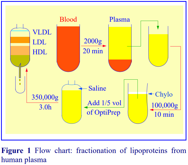 processing it is often necessary to remove the salt by dialysis, often adding a further 12 h to the procedure. Moreover, the use of high salt concentrations may cause the removal of surface apolipoproteins from lipoproteins.
Self-generated gradients iodixanol in vertical or near-vertical rotors (3-12 ml tubes) considerably simplify the separation procedure [1,2]. After removal of chylomicrons, plasma is adjusted to a suitable starting density by addition of a small volume of OptiPrep; loaded into a centrifuge tube and centrifuged for 2-3 h. The procedure is summarized in the flow chart that is Figure 1.
♦ This Application Sheet describes the basic technique. For some of the possible variations in gradient conditions, which may be more appropriate to subfractionation of lipoprotein classes, see Application Sheet M08.
There are some significant advantages to the use of self-generated gradients over the more traditional sequential flotation methods
♦ Ease of sample handling
♦ Shorter separation times reduce possible cholesterol oxidation
 2. Solutions required
A. OptiPrep™
B. Hepes-buffered saline: 0.85% (w/v) NaCl, 10 mM
Hepes-NaOH, pH 7.4
3. Ultracentrifuge rotor requirements
Any vertical, near-vertical or small volume fixed angle rotor (sedimentation path length of approx 17 mm or less) for an ultra- or microultra- centrifuge. Tube volumes of 2-12 ml are normally suitable. Most studies have been carried out using the following Beckman rotors: TLN100 near-vertical, VTi65.1 vertical, NVT65 near-vertical and NVT65.2 nearvertical (see Note 1) but others such as the TLV-100, and NVT90 will give similar separations. Sorvall ultracentrifuge vertical rotors such as the TV865, TV1665, Stepsaver™ 65V13, Stepsaver™ 70V6 and microultracentrifuge rotors such as the S120-VT and RP100-VT are alternatives.
4. Protocol (for 3.3 ml tubes in the Beckman TLN100 near-vertical rotor)
1. Using freshly drawn blood (1 mM EDTA as anti-coagulant), pellet the cells at 2000 g for 15 min (see Notes 2 and 3).
2. Remove chylomicrons from the plasma by centrifugation at 100,000 g for 10 min (see Note 4).
3. Mix 4 vol of plasma with 1 vol of OptiPrep™ (12% iodixanol final concentration) and transfer 2.8 ml to an OptiSeal™ tube (see Note 5).
4. Layer Solution B on top to fill the tube (see Notes 6 and 7).
5. After sealing the tube, centrifuge at approx 350,000 gav for 2.5-3 h at 16°C, using slow acceleration to and deceleration from 2000 rpm.
6. Collect the gradient in 0.1 – 0.2 ml fractions by tube puncture and analyze the fractions (see Notes 8-13).
5. Notes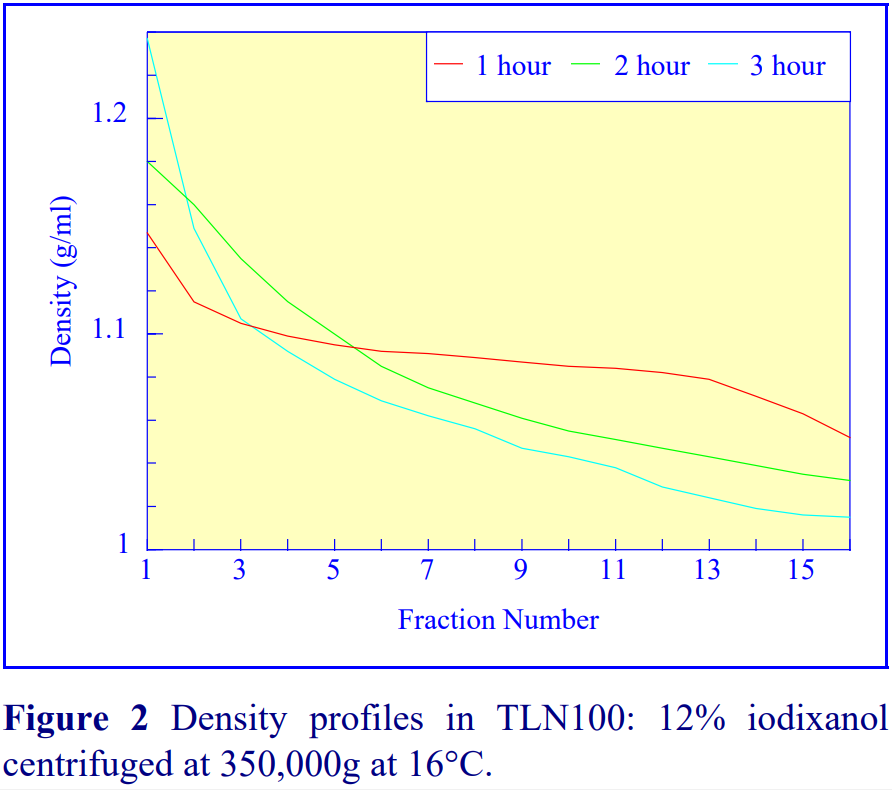 1. The gradient density profiles obtained after 2-3 h in the TLN100 near vertical rotor (Figure 2) are the most useful for the majority of lipoprotein separations, although the S-shaped profiles (obtained after 1 h) containing a shallow median section might be adapted to lipoprotein subfractionation, so long as this is sufficient time for the lipoproteins to reach their banding density. For more information on the formation of self-generated gradients see Application Sheet M03.
2. Citrate may also be used as anticoagulant; heparin has not been tested. Serum may be used instead of plasma.
3. For species other than human go to the AxisShield Abstract Database (see Section 8).
4. The conditions used to float chylomicrons vary widely, the higher g-forces for shorter times used here are very effective.
5. Other concentrations of iodixanol may be suited to the purification of specific lipoproteins and for plasma from other species.
6. The saline on top of the sample not only conveniently fills the tube; it minimizes the tendency of the VLDL to adhere to the wall of the tube. This is particularly important with vertical rotors. It also enhances the separation of the VLDL from the lightest LDL in all rotors.
7. In vertical rotors it may also be beneficial to include a small volume of 20% iodixanol (approx 0.5 ml) as a cushion to prevent soluble proteins sedimenting on to the outer side of the tube This is less important in near-vertical or fixed-angle rotors.
8. Tube puncture generally provides a better recovery of VLDL from an Optiseal tube than does upward displacement. On the other hand the plasma proteins at the bottom of the tube tend to contaminate the dense HDL fractions more seriously if tube puncture is used. For more information on harvesting gradients see Application Sheet M04.
9. Fractions from iodixanol gradients can be analyzed directly by agarose gel and SDS-PAGE electrophoresis and for cholesterol and triacylglycerol without dialysis of the medium. Iodixanol is non-ionic and does not interfere with any of these analytical procedures. A typical agarose gel is shown in Figure 3.
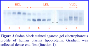 10. The banding densities of LDL and particularly HDL, are lower than in salt gradients. In iodixanol gradients apolipoproteins retain any bound water. In hyperosmotic salt gradients this water is lost (see ref 2 for more details).
11. Not only is excellent resolution achieved of the major classes of lipoprotein, the method also produces a significant concentration of the lipoproteins. A typical agarose gel electrophoresis profile of a gradient is shown in Figure 3. From each fraction, 3 µl was applied directly to a commercial agarose gel and after electrophoresis was stained in Sudan black.
12. Application Sheet M08 describes some of the modifications to the gradient system that can be used in analysis of the sub-classes of lipoproteins.
13. If the separation is carried out in a tube for the VTi65.1 vertical rotor, the tall format of this tube promotes the maintenance of the resolving power of the gradient during unloading.
♦ There are a number of published reviews on the gradient technology used for plasma lipoprotein fractionation and these are listed below in Section 6 [3-6]. Some of these also provide an overview of other methodologies and ref 5 describes the adaptation of the methodology described above to the use of larger volumes of plasma.
6. References
1. Graham, J.M., Higgins, J.A. and Gillot, T. (1995) A new method for the rapid separation of plasma lipoproteins Atherosclerosis, 115 (Suppl), S123
2. Graham, J., Higgins, J. A., Gillott, T., Taylor, T., Wilkinson, J., Ford, T. and Billington, D. (1996) A novel method for the rapid separation of plasma lipoproteins using self-generated gradients of iodixanol Atherosclerosis, 124, 125-135
3. Patterson, B. W. (2002) Methods for measuring lipid metabolism in vivo Curr. Opin. Clin. Nutr. Metab. Care, 5, 475-479
4. Langlois, M.R. and Blaton, V.H. (2006) Historical milestones in measurement of HDL-cholesterol: Impact on clinical and laboratory practice Clin. Chim. Acta, 369, 168-178
5. Billington, D., Maxwell, E., Graham, J.M. and Newland, P. (2007) Large-scale preparation of human low- and highdensity lipoproteins by density gradient centrifugation using iodixanol Anal. Biochem., 367, 137-139
6. Yee, M.S., Pavitt, D.V., Tan, T., Venkatesan, S., Godsland, I.F., Richmond, W. and Johnston, D.G. (2008) Lipoprotein separation in a novel iodixanol density gradient, for composition, density and phenotype analysis J. Lipid Res., 49, 1364-1371
OptiPrep Application Sheet M07; 6th edition, Jan. 2020
OptiPrep™ Application Sheet M08
Analysis of mammalian and non-mammalian HDL, LDL and VLDL
- OptiPrep™ is a 60% (w/v) solution of iodixanol in water; density = 1.32 g/ml
- The basic methodology was developed for human plasma but it has subsequently been extended to other species and also used for human Coomassie blue-stained lipoproteins
- The OptiPrep™ Reference List “Fractionation of plasma lipoproteins” (RM01) provides a comprehensive bibliography of all the published papers (nearly 100) reporting the use of OptiPrep™: to access RM01 return to the initial list of Folders and select “Reference List”
- To access other Application Sheets referred to in the text: return to the 2020Macroapp file and select the appropriate M-number.
1. Background
In the routine method, chylomicron-free plasma is adjusted to 12% (w/v) iodixanol and the sample, essentially fills an approx 3 ml tube for a near-vertical rotor. During the centrifugation VLDL, LDL and HDL particles and also plasma proteins migrate from all parts of the sample to their final buoyant density banding position in the self-forming density gradient. This method was developed with the Beckman TLN100 near-vertical rotor – see Application Sheet M07.
By modulating the experimental conditions in a variety of ways it is possible to influence the profile of the density gradient that is formed during the centrifugation and thus alter the linear resolution of the various lipoprotein fractions within the tube. The profile is modulated by:
- Small changes to the centrifugation time and iodixanol concentration.
- Choice of rotor; the recommended Beckman rotors (TLN100, VTi65.1, NVT65, NVT65.2) have similar but not identical sedimentation path lengths; the density gradient profile generated from the same concentration of iodixanol at the same gav and centrifugation time, is consequently sufficiently different in each rotor type to affect the resolution of the lipoproteins.
- Tube loading format; unique density profile modulations can be achieved by using a two layer format (e.g. equal volumes of 12% (w/v) and 6% (w/v) iodixanol) rather than a single uniform concentration.
The effect of iodixanol concentration and tube-loading format, in the NVT65.2 is given in Figure 1. Panel 1 shows the banding of the major lipoproteins using the same tube format, centrifugation time and RCF as described in Application Sheet M07; the only difference is the rotor type (results from a TLN100 are shown in Figure 3 of M07. In the NVT65.2 the gradient density profile causes the HDL to band more broadly (and the LDL more sharply) across the gradient fractions than in the TLN100. There is even some indication that the use of a uniform concentration of 12% iodixanol at 365,000g for 3 h in the NVT65.2 rotor may permit the resolution of the HDL into distinct subfractions; the three boxed fractions in Panel 1 clearly indicate a minor population of HDL particles denser than the major population. Only by reducing the uniform iodixanol concentration to 9% in the NVT65.2 (Panel 2), does the relative linear distribution of the HDL and LDL approach that obtained with 12% iodixanol in the TLN100.
Panel 3 shows the distribution of lipoproteins in a two layer tube-loading format of 12% and 9% iodixanol (equal volumes of each) with the plasma confined to the denser layer. It might be expected that the gradient generated from the 12% iodixanol in the bottom half of the tube would have caused the HDL to band further up the tube when compared to the banding in a gradient generated from a uniform 9% iodixanol format (Panel 2). The important consideration here is the amount of plasma proteins in the system; plasma proteins contribute significantly to the total density of the gradient, particularly in the lower half of the gradient. The 12%/9% format contains less than half of the plasma

proteins present in the 9% format; moreover in the two layer format, the proteins molecules, already restricted to the lower half of the tube, also sediment more effectively towards the bottom of the tube.
2. Fractionation of LDL subclasses
Subfractionation requires an increase in the resolving power of the gradient, not only to aid identification and quantitation of LDL subclasses in a reproducible manner, but also to improve the linear separation of dense LDL from lighter HDL. This can be achieved in a number of ways (see above and ref 1 for more details).
- By confining the plasma sample to a dense load zone (12% iodixanol) at the bottom of the tube and layering a solution of 9% (or sometimes 6%) iodixanol in saline on top, the HDL and plasma proteins sediment through the gradient formed within the 12% layer while the LDL (and VLDL) particles float (and band) in the “clean” gradient formed by the 9% layer.
- The profile of the low density resolving gradient can be adjusted by changing the relative volumes of the high and low density layers and by changing centrifugation time.
- The use of a larger volume tube of sedimentation path length similar, but not identical, to that of the TLN100 (i.e. a taller tube) may enhance the effect of these modulations.
- Harvesting the gradient in a larger number of small volume fractions will also better maintain the fractionation achieved by the gradient.
The following protocol provides a basic strategy (adapted from refs 1 and 2). In the Notes are some recommendations from published papers for optimizing the resolving power and/or for alternative analytical procedures.
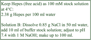 2a. Solutions required
A. OptiPrep™
B. Hepes-buffered saline: 0.85% (w/v) NaCl, 10 mM
Hepes-NaOH, pH 7.4
C. Cholesterol analysis kit
Figure 1 Sudan black stained agarose gel electrophoresis profiles of human plasma lipoproteins. Panel 1, 12% iodixanol; panel 2, 9% iodixanol; panels 3, 12%/9% iodixanol. All gradients were centrifuged in 5.1 ml tubes in the Beckman NVT65.2 near-vertical rotor at 350,000 g for 3h. All gradients were unloaded dense-end first. See text for more details Keep Hepes (free acid) as 100 mM stock solution at 4°C:
2b. Ultracentrifuge rotor and gradient harvesting requirements
Beckman near-vertical rotor; TLN100, NVT65.2 or NVT65 (see Note 1)
Beckman Fraction Recovery System (for tube puncture) or Labconco Auto Densi-Flow™ gradient collector (for collection from the meniscus) (see Note 2)
Peristaltic pump and fraction collector (to take 96 well microtitre plate)
2c. Protocol (for TLN100 rotor)
1. Using freshly drawn blood (1 mM EDTA as anti-coagulant), pellet the cells at 2000 g for 15 min.
2. Remove chylomicrons from the plasma by centrifugation at 100,000 g for 10 min (see Note 3).
3. Mix 4.25 vol. of Solution B with 0.75 vol. of OptiPrep™ (9% iodixanol final concentration) and transfer 1.4 ml to an OptiSeal tube for a Beckman TLN100 rotor (see Notes 4-6).
4. Mix 4 vol. of plasma with 1 vol. of OptiPrep™ (12% iodixanol final concentration) and use 1.4 ml to underlayer the 9% iodixanol solution (see Notes 4 and 5).
5. Layer Solution B on top to fill the tube (see Note 6).
6. After sealing the tube, centrifuge at approx 350,000 gav for 2.5-3.0 h at 16C, using slow acceleration to and deceleration from 2000 rpm (see Note 7).
7. Collect the gradient in 0.07-0.1 ml fractions by tube puncture into a 96 well microtitre plate and analyze the fractions for cholesterol (see Notes 8-13).
2d. Notes
1. Near-vertical rotors are the preferred type since the soluble proteins sediment towards the bottom of the tube (like a pellet in a fixed-angle rotor). In a vertical rotor the proteins will sediment on to the wall of the tube, down the length of the tube, unless a small volume (0.2 ml) of 20% iodixanol is included. See ref 1 for more information on the use of other rotors.
2. Collection from the meniscus is the preferred method because in tube puncture the first few fractions containing soluble plasma proteins are very viscous and tend to contaminate the succeeding densest HDL fractions.
3. Lower speeds for longer times may be used.
4. Alternatively overlayer the plasma with the 9% (w/v) iodixanol; sometimes 6% iodixanol is used.
5. The relative volumes of the plasma in 12% and the 9% iodixanol can be adjusted to suit the tube volume. Davies and Griffin [3] for example used 3 ml of plasma and 8 ml of 9% iodixanol in an NVT65 rotor. Larger volume tubes, in which the volume of the resolving gradient can be increased, potentially provide an improved resolution over the smaller volume tubes.
6. The saline on top of the sample not only conveniently fills the tube, it minimizes the tendency of the VLDL to adhere to the wall of the tube. This is particularly important with vertical rotors. It also enhances the separation of the VLDL from the lightest LDL in all rotors.
7. Sawle et al [2] found that 2.5 h (in the TLN100) gave a better resolution of the denser LDL from the lighter HDL; this is due to the slightly steeper gradient (in the top 2/3rds of the tube) at the shorter time. It is advisable to test the optimum time (in the 2.5-3.0 h range) for other rotor types.
8. Because iodixanol absorbs strongly in the UV it is not feasible to monitor the lipoprotein distribution in the gradient by direct spectrophotometric measurement. As an alternative to monitoring the cholesterol content of the collected gradient fractions, Davies and Griffin [3] prestained the plasma with Coomassie blue (see Note 12).
9. An example of the resolution achievable with the TLN100 is given in Figure 2. The three plasma samples exhibited distinctive LDL distributions with peak LDL densities in fractions 5, 6 or 8 (in a 19 fraction gradient harvest). By reducing the centrifugation time to 2.5 h and taking smaller fractions (44 in total) it is possible to detect differences in LDL banding more easily [2]; under these conditions the peak positions can differ by as many as 10 fractions.
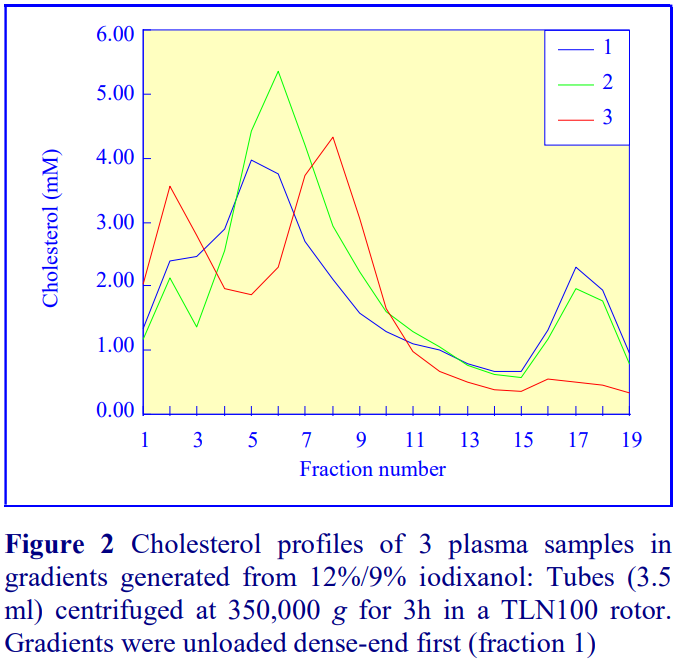 10. The methodology for determining the LDL density banding profile using iodixanol gradients has now been validated against other techniques
11. Sawle et al [2] improved the resolution significantly by decreasing the fraction volume size and collected a TLN100 gradient in 44 fractions.
12. If the lipoproteins are pre-stained with Coomassie blue [3,4], it is possible to short-cut the need to unload the gradient by taking a digital photograph of the tube. After downloading on to a PC, the image is analyzed by computerized gel scanning technology to obtain a profile of the Coomassie blue staining. The method has been validated against the established KBr gradient technology.
13. Any lipid analysis or gel electrophoresis can be carried out directly on the gradient fractions. If it is necessary to remove contamination of HDL fractions by plasma proteins, centrifuge the gradient sample through an ultrafiltration cone with a 100 kD mol wt cut-off (e.g. Whatman Vectaspin 3TM polysulphone centrifuge tube filter).
3. Fractionation of HDL subclasses
The use of iodixanol gradients to fractionate HDL subclasses from pre-stained plasma has been reported by Harman et al [5,6].
- There are also a couple of published reviews on the gradient technology used for LDL subclass fractionation [7,8]; they also provide an overview of other methodologies.
4. References
1. Graham, J.M., Griffin, B.A., Davies, I.G. and Higgins, J.A. (2001) Fractionation of lipoprotein subclasses in selfgenerated iodixanol gradients In Methods Mol. Med., 52, Atherosclerosis, experimental methods and protocols (ed Drew, A.F.), Humana Press, Totowa, NJ. pp 51-59
2. Sawle, A., Higgins, M.K., Olivant, M.P. and Higgins, J.A. (2002) A rapid single-step centrifugation method for determination of HDL, LDL, and VLDL cholesterol, and TG, and identification of predominant LDL subclass J. Lipid Res., 43, 335-343
3. Davies, I.G. and Griffin, B.A. (2001) Rapid identification of LDL subclass phenotypes by iodixanol gradient centrifugation Atherosclerosis, 159, 249
4. Davies, I.G., Graham, J.M. and Griffin, B.A. (2003) Rapid separation of LDL subclasses by iodixanol gradient ultracentrifugation Clin. Chem., 49, 1865-1872
5. Harman, N.L., Davies, I.G. and Griffin, B.A. (2007) Separation of the principal HDL subclasses by iodixanol gradient ultracentrifugation Atherosclerosis, 194, 283
6. Harman, N.L., Griffin, B.A. and Davies, I.G. (2013) Separation of the principal HDL subclasses by iodixanol ultracentrifugation J. Lipid Res., 54, 2273-2281
7. Chung, M., Lichtenstein, A.H., Ip, S., Lau, J. and Balk, E.M. (2009) Comparability of methods for LDL subfraction determination: A systematic review Atherosclerosis 205, 342–348
8. Hirayama, S. and Miida, T. (2012) Small dense LDL: An emerging risk factor for cardiovascular disease Clin. Chim. Acta, 414, 215–224
OptiPrep™Application Sheet M08; 8th edition, January 2020
OptiPrep™ Application Sheet M09
Analysis of protein complex formation, microtubules and cytoskeleton
- OptiPrep™ is a 60% (w/v) solution of iodixanol in water, density = 1.32 g/ml
- To access other Application Sheets referred to in the text: return to the 2020Macroapp file and select the appropriate M-number.
1. Background
Determination of the sedimentation coefficient of a protein, traditionally in a 5-20% sucrose gradient, in order to determine its molecular mass, is a technique that was developed many years ago. Although alternative methods, notably polyacrylamide gel electrophoresis, have achieved a wide popularity, there are certain situations that are better suited to density gradients, for example the analysis of heavily glycosylated proteins, which run anomalously on gels. Another area that may be better suited to density gradient analysis is the study of protein-protein interactions. The standard sucrose gradient analysis, which is carried out in swinging-bucket rotors for 4-16 h, may be less than ideal for determining protein-protein interactions. Macromolecular complexes may be insufficiently stable to survive these long centrifugation times and they may be intolerant of the high hydrostatic pressures generated in a swinging-bucket rotor [1,2]. In addition Timasheff [3] pointed out that solutions of low water activity (high osmolality) can remove bound water from proteins and could cause changes in stability of the protein and its propensity to aggregate. The use Nycodenz will reduce the osmolality (raise the water activity) of gradients considerably, while with iodixanol gradients can be made isoosmotic throughout the entire useful density range. Gradient made from one or other of these solutes may therefore be an important advantage in studying protein-protein interactions in density gradients. Some reports also highlight the functional problems associated with sucrose gradients; for example these caused proteolysis of a kinesin-related motor protein, while in iodixanol gradients there was no proteolysis whatsoever [4]. This Application Sheet covers the following topics:
- Section 2: Alzheimer’s Aβ peptide and other neurodegenerative disease-associated proteins
- Section 3: Non-muscle myosin II (NMII)
- Section 4: Dimerization of the kinesin-related motor protein KIF1A
- Section 5: α-Synuclein aggregation
- Section 6: Microtubule fragment size analysis
- Section 7: Cytoskeleton analysis
- Section 8: Prion proteins and fibrils
- Section 9: Association of Drosophila proteins with lipophorin
- Section 10: Hepatitis and Herpes virus proteins
- Section 11: Other recent applications
2. Alzheimer’s disease amyloid-beta (A) peptide
2a. Aggregation (oligomerization) studies
2a-1. Introduction
Moir et al [5] studied the aggregation of the Aβ peptide by Zn2+, Cu2+, EDTA or a pH 5.5 buffer. The incubations were simply layered over a series of NycodenzⓇ barriers of increasing density; the concentrations were 43%, 44%, 44.6%, 46.8% and 47% (w/v) in microcentrifuge tubes and centrifuged at 16,000 g for 10 min. Tubes were then analyzed by rapid freezing to -170°C for 1 h and “fractionated” by cutting the tube. All the treatments, except EDTA, allowed the aggregates to sediment through the 43 and 44% barriers but only the Zn2+ induced aggregates sedimented through the 44.6 and 46.8% barriers.
The analysis of oligomerization of the -amyloid A peptide in iodixanol gradients, using a high performance near-vertical rotor, developed by Ward et al [6], may be applicable to any protein oligomerization studies and is thus given here in some detail. The short sedimentation path length of the rotor (18 mm) means that the centrifugation time can be reduced to 3 h and the hydrostatic pressure is correspondingly low. The authors used the gradients to analyze the interactions of the β amyloid (Aβ) peptide that is implicated in Alzheimer’s disease, but the strategy could be used or adapted to any protein oligomerization or protein-protein interaction study. The protocol described below is adapted from ref 6. For Notes see Section 2a-5
2a-2. Solutions required
A. OptiPrep™
B. OptiPrep™ diluent: for the study of the oligomerization of β-amyloid (Aβ) peptide [6] the diluent used was phosphate-buffered saline (PBS), but any diluent compatible with the protein-protein interaction may be used (see Note 1). Include protease inhibitors in solutions as required.
2a-3. Ultracentrifuge rotor requirements
A near-vertical (e.g. Beckman NVT100, NVT90 or NVT65.2) or vertical (e.g. Beckman VTi90, VTI65.2 or Sorvall TV1665 or 70V6) rotor: all these rotors accommodate tubes for approx 5 ml total volume (see Note 2).
2a-4. Protocol
1. Carry out all operations at 0-4°C or any temperature compatible with the interactions under investigation.
2. Dilute OptiPrep™ with PBS to produce the solutions used in the next step (see Note 1).
3. Layer sequentially in tubes for the chosen rotor: 0.65 ml of 50%, 40% and 30% (w/v) iodixanol, 1.95 ml of 20%, 0.65 ml of 10% and 0.3 ml of 5% (w/v) iodixanol (see Note 3)
4. Layer 0.3 ml of the protein solution on top and centrifuge at 350,000 g for 3 h at 0-4°C, using controlled acceleration and deceleration over the 0-2000 rpm range (see Note 4).
5. Collect the gradient in 0.3-0.35 ml fractions either by upward displacement with Maxidens™ and an Axis-Shield Gradient Collector, tube puncture or by automatic aspiration from the meniscus using a Labconco Auto Densi-flowⓇ (see Notes 5 and 6).
- See Notes 7-11 for other examples of the use of iodixanol gradients for Aβ peptide studies
2a-5. Notes
1. If it is important to maintain a constant background of buffer concentration (e.g. 20 mM Tris-HCl, pH 8.0) and low concentration of some other additive (e.g. 1 mM EDTA and 1 mM DTT); then a 50% (w/v) iodixanol working solution (WS) should first be prepared by mixing 5 vol. of OptiPrep™ with 1 vol. of 6 mM EDTA, 6 mM DTT, 120 mM Tris-HCl, pH 8.0. Further dilutions are then obtained by dilution of the WS with 20 mM Tris-HCl, pH 8.0, 1 mM DTT, 1 mM EDTA. All gradient solutions will then contain the requisite concentration of buffer and additive. For more information on the preparation of density gradient solutions see Application Sheet M01.
2. Vertical or near-vertical rotors are ideal for sedimentation velocity separations because, (a) the sample layer achieves a very narrow zone-width after reorientation and (b) the sedimentation path length is short. If other rotors (fixed-angle or swinging-bucket) are used the sample volume must never be greater than 10% of the gradient volume and the centrifugation time will need increasing to take account of the longer sedimentation path length (particularly in larger volume swingingbucket rotors).
3. Because of the short path length, the gradient will become more or less continuous within 30 min. An alternative approach may be to produce a
linear continuous gradient in the centrifuge tube before layering the sample (see Application Sheet M02); however the irregular density profile achieved by using the non-uniform layer volumes described in Step 3 of the Protocol will be lost. The consequences of this are not clear.
4. If the method is being used to study the oligomerization of other proteins the RCF or centrifugation time may need modulation according to the size of the protein particles.
5. An example of the resolution, which is achievable with this gradient system, is given in Figure 1. Freshly-prepared hexafluoro-2-propanol (HFIP) treated -amyloid (A) peptide oligomerizes during incubation at 35C and the distribution of this peptide across the gradient was analyzed by SDS-PAGE after 0 min, 30 min, 18 h and 18 days of incubation at this temperature. The position of the peptide in the gradient reflects the extent and type of association of the peptide monomers.
6. For more information on methods of harvesting gradients see Application Sheet M04.
7. The method has also been adapted to small volume swinging-bucket rotors: Rzepecki et al [7] used a similar gradient, which was scaled down to use in a Beckman TLS55 (2.2 ml tubes) with centrifugation at 259,000 g for 4 h and Lockhart et al [8] used a Beckman MLS50 (5 ml tubes) for studying the formation of -amyloid fibrils at 268,000 g for 3 h. The Rzepecki et al [7] gradient was also used by Funke et al [9] to study the effect of the D-enantiomeric peptide D3, which caused a shift of the A peptide from an oligomeric form to much larger aggregates and the A binding peptide L3 [10].
8. More recent studies of the oligomerization procedure [11-13] have also used the TLS55 rotor under more or less similar centrifugation conditions; the gradients were however slightly modified; a discontinuous gradient of 0.26 ml each of 50%, 40% and 30% iodixanol, 0.78 ml of 20%, 0.26 ml of 10% and 0.1 ml of 5% iodixanol. The gradients were used to analyse Aβ (1-42) aggregates using 100l of samples, which was layered on top. The gradient system described by Brener et al [11] has been used to show the preferential binding of monomeric Aβ to D-peptides [13-16] and GM1 [17].
9. Sehlin et al [18] used an iodixanol gradient similar to that of Ward et al [6] each step was 0.65 ml except for the 30% (w/v) iodixanol (1.95 ml) and omitted the 5% layer. The gradient effectively resolved A peptide aggregates of different sizes.
10. A prions have also been extensively purified in a multi-step method. In the primary fractionation of a brain homogenate the latter was adjusted to 18% (w/v) iodixanol and layered over 30% and 35% iodixanol. After centrifugation at 60,000 g for 20 min the top lipid layer was discarded and the material within the denser two layers collected. After dilution with buffer, this was layered over a second gradient of 26% and 35% iodixanol and centrifuged at the same speed for 40 min. Again the top layer was discarded and the material in the two denser layers recovered prior to further processing [19].
11. More recently a simple discontinuous flotation gradient (36%, 24% and 0% iodixanol) centrifuged at 54,000 g for 3 h was used to separate less dense LDL-bound Aβ from Aβ [20].
12. Iodixanol gradients have recently been used to purify metal nanoparticle-conjugated Aβ-specific ligands to increase binding affinity.
2b. Other neurodegenerative disease-related protein studies
2b-1. Fibrillar structures
Levy et al [22] adapted the method described in Section 2 to an analysis of islet amyloid fibril formation using a 3 ml pre-formed continuous 0-60% (w/v) iodixanol gradient, generated from equal volumes of OptiPrep and water (pH 2) in tubes for a Beckman SW60Ti swinging-bucket rotor. The gradients were loaded with 0.6 ml of sample and centrifuged at 150,000 g for 24 h. The gradient separated a series of low molecular mass pre-fibrillar assemblies in the top half of the gradient from the fibrils at the bottom. More recently Frenzel et al [23] separated fibrils from smaller aggregates and monomers by iodixanol density gradient centrifugation. The gradient comprised layers of 50%, 40%, 30%, 20%, 10% and 5% (v/v) OptiPrep iodixanol in 10 mM phosphate buffer pH 7.4; the sample was top-loaded. Centrifugation in a small volume (2.2 ml tubes) swinging-bucket rotor for 3 h at 259,000 g, resolved the three forms of the protein.
- See Section 3 for a related method for separating monomeric and filamentous protein forms.
The method developed by Ward et al [6] has been adapted to the slightly larger tubes (6 ml) of the Sorvall TV865 by Khlistunova et al [24] for studying the Tau protein; usually a soluble protein, but in some neurodegenerative diseases it forms “paired helical filaments” and associates with microtubules. The gradient was generated from 0.85 ml of 50% and 40%, 2.2 ml of 30%, 0.85 ml of 10% and 0.3 ml of 5% (w/v) iodixanol. Sarcosyl-insoluble fractions from neuronal tissue have also been purified in an iodixanol gradient [25]. Gradients covering approx. the same density range (145,000 g for 12 h) have analyzed the association between Tau and a 14-3-3 protein [26].
3. Non-muscle myosin II (NMII)
This investigation was reported by Shutova et al [27]. Detergent-soluble cell lysates was layered on to a discontinuous gradient of 50%, 25%, 12%, and 6% OptiPrep layers. After centrifugation at 80,000 rpm for 1 h the gradient resolved monomeric and filamentous forms of NMII which had sedimentation coefficients of approx 7S and 16S respectively. The monomeric form was found to be increased to a greater extent in blebbistatin-treated cells. The same gradient was reported in ref 28.
4. Kinesin-related motor protein KIF1A dimerization
Rashid et al [4] used a 3.8 ml continuous gradient of 5-40% (w/v) iodixanol overlaid by 0.2 ml of sample in a Beckman SW60Ti swinging-bucket rotor at 100,000 gav for 16 h at 4C, to identify dimers of KIF1A.
5. -Synuclein aggregation
Rather larger protein aggregates of cytoplasmic -synuclein from COS7 cells have been analyzed in discontinuous gradients of 2.5%, 25% and 35% (w/v) iodixanol, centrifuged at only 50,000 g for 30 min [29].
6. Microtubule fragment size analysis
MacCormick et al [30] characterized a large protein complex containing a nerve-growth-factoractivated ERK (extracellular-signal-regulated kinase) and MEK. Part of the fractionation process included the isolation of a non-ionic detergent insoluble fraction that also contained microtubule fragments that contained some bound kinases. Glycerol gradients were not effective in resolving the larger microtubule fragments; the following iodixanol gradient method devised by MacCormick et al [30] however provided excellent resolution of these particles.
1. Permeabilize PC12 cells by a single passage through a ball-bearing homogenizer.
2. Release the intracellular material by the permeabilization and separate from the residual “cells” by centrifugation at 1000 g for 10 min.
3. Concentrate the supernatant material by pelleting at 100,000 g through a cushion of 10% (w/v) sucrose in 20 mM MOPS (pH 7.2) containing 1 mM EGTA and 1 mM Na3VO4.
4. Suspend the pellet in buffer containing potassium aspartate, potassium gluconate and potassium glutamate (all 38 mM), 20 mM MOPS, 10 mM potassium bicarbonate, 0.5 mM magnesium carbonate, 1 mM EDTA, 1 mM EGTA, pH 7.1.
5. Prepare a 30% (w/v) iodixanol solution in the same buffer and make a continuous 0-30% iodixanol prepared using a two-chamber gradient maker or Gradient Master. If neither of these devices is available make up a discontinuous gradient from equal volumes of 0%, 10%, 20% and 30% (w/v) and allow to diffuse overnight at 4C. For more information about preparing continuous iodixanol gradients see Application sheet M02.
6. Layer the sample on top of the gradient (sample volume <10% of total gradient volume). The gradient separation is a sedimentation velocity one, so its resolving power is inversely proportional to the sample volume. Centrifuge at 200,000 g for 1-3 h (turn off the brake during deceleration from 2000 rpm or use a controlled deceleration program).
7. Collect the gradient either by tube puncture or collection from the meniscus. For more information about gradient fractionation see Application Sheet M05. MacCormick et al [30] collected the gradient in 27 fractions.
- After a centrifugation for 1 h the microtubule fragments from PC12 cells has been resolved on the basis of size into four discrete fractions, as determined by the -tubulin distribution [30] but ERK was only associated with three of them.
7. Cytoskeleton analysis
Plasma membrane and cytoskeleton in Drosophila extracts have been effectively separated on 10- 40% (w/v) iodixanol gradients prepared by dilution of OptiPrep with 0.25 M Sucrose, 10 mM TrisHCl, pH 8.0 centrifuged at 250,000 g for 3 h [31]. It provided a very clear separation of the syntaxin 1A (plasma membrane marker) the denser myosin II heavy chain (cytoskeleton marker).
A widely used discontinuous sedimentation velocity gradient originally devised by Majoul et al [32], comprising 2.5%, 5%, 7.5%, 10%, 12.5%, 15%, 17.5%, 20%, and 30% (w/v) iodixanol was used by Chen et al [33] who studied the cytoskeleton structure in a 65,000 g (1 h) fraction from a postnuclear supernatant of a mouse spinal cord homogenate. The gradients were allowed to diffuse at 4C for 3-4 h solution before loading the fraction and centrifuging at 170,000 g for 90 min. Both actin and tubulin showed a biphasic distribution, being concentrated in the top quarter of the gradient but also demonstrating a sharp band about three-quarters of the way down the gradient. Mice deficient in a presenilin binding protein called “modifier of cell adhesion” (MOCA) lacked the sharp denser band. Cofilin-actin rods have been isolated from cultured nerve cells in a double gradient strategy [34]. All steps were performed at 4C. A low-speed supernatant was layered over 10% and 15% (w/v) iodixanol and centrifuged at 6,650 g for 10 min to band the rods above the interface between the two iodixanol layers. The collected fraction was diluted with 13% iodixanol (vol. ratio of approx 0.4:1.7) and centrifuged at 166,000 g for 2 h to create a self-generated gradient – a small volume vertical rotor is best suited to self-generated gradient formation (see OptiPrep Application Sheet M03 for more information on self-generated gradients). The rods band close to the bottom of the gradient. Once recovered, the rods in the fraction (after dilution with an equal volume of buffer) may be concentrated on a 25% iodixanol cushion at 5,000 g for 15 min [33]. Actin rods have also been analyzed on a twolayer gradient (10% and 15% v/v OptiPrep, centrifuged at 6,600 g for 10 min [35].
Phosphorylation of the vasodilator-stimulated phosphoprotein (VASP) controls its influence on Factin-related processes and Lin et al [36] studied them in Dictyostelium. A discontinuous iodixanol gradient of 5%, 10%, 15% and 20% (w/v) iodixanol centrifuged at approx 150,000 g for 18 h. WASP banded broadly in the bottom half of the gradient but in the presence of VASP, the WASP distribution shifted significantly to a higher density.
8. Prion proteins
Tixador et al [37] solubilized the proteins from a mouse brain homogenate in a buffered solution of dodecyl--D-maltoside and N-lauryl sarcosine. The material was layered on top of a continuous 10- 25% (w/v) iodixanol gradient (4.8 ml total volume) and centrifuged 285,000 g for 45 min. The hostencoded prion protein (PrPC) banded close to the top of the gradient, while the PrPSc, the multimeric misfolded conformer PrPSc banded about half-way down the gradient. Discontinuous iodixanol gradients have also been used as part of the procedure in the purification of prion fibrils from mouse brain [38]. Sarcosyl-containing 10-54% (w/v) iodixanol gradients (200,000 g for 1 h) have also been used to determine the size of aggregates containing prion protein [39].
An extensive study of the quaternary structure of prion proteins was carried out by Laferriè et al [40] using both sedimentation velocity and equilibrium iodixanol density gradients. Mouse brain homogenates were solubilized in a buffered saline containing EDTA, DTT, dodecyl--D-maltoside and N-lauryl sarcosine.
- For sedimentation velocity analysis the samples were layered on top of a continuous 10–25% iodixanol gradient and centrifuged at 285 000 g for 45 min. In some studies the time was increased to 90 min; this provided additional resolution of the proteins. Rapidly- and slowly-sedimenting ovine strains were identified
- For equilibrium gradients the sample was adjusted to 40% iodixanol and made part of a discontinuous gradient spanning the range 10-60% iodixanol and centrifuged at 115,000 g for 17 hours.
- Similar sedimentation velocity gradients (5-25% iodixanol) were used by Coleman et al [41] in the identification of small soluble protease-sensitive prion proteins as the major source of infectivity in mouse brain.
- Wenborn et al [42] were able to purify prion protein from brain homogenates that was devoid of ferritin and other contaminating proteins by a combination of filtration and a series of centrifugations through 17.5% (w/v) iodixanol at 16,100 g.
- Herrmann et al [43] used 10-40% and 2-20% iodixanol gradients (52,000 rpm for 90 min) to show an impoverishment of the larger molecular weight prion proteins (from mouse brain) during drug treatment.
- Sarkosyl-solubilized brain material has been analyzed [44] in a 7-28% OptiPrepTM gradient (18,000 g for 20 min) and solubility assays were carried out in 15% OptiPrepTM at 18,000 g for 30 min [45, 46].
- Most recently, sedimentation velocity analysis has been carried out on 150 μl of a sarkosylsolubilized fractions loaded on to 4.8 ml 10-30% iodixanol gradients centrifuged at 285,000 g for 45 min [47].
9. Association of Drosophila proteins with lipophorin
This methodology was first reported by Eugster et al [48]: a homogenate of larvae was centrifuged at 120,000 g and the supernatant adjusted to adjusted to 50% (w/v) iodixanol and layered beneath gradients of 10%–20% to 35%–45% (w/v) iodixanol. They were centrifuged at 4C, at 285,000 g, for 16 h in a swinging-bucket rotor (2.2 ml tube volume). There is no obvious reason why the separation cannot be scaled up. Proteins not bound to the lipophorin lipoprotein remained at the bottom of the gradient, while lipophorin- bound proteins floated into the top half of the gradient. The method was used to study the interaction of the lipophorin with various morphogens via heparan sulphate. Similar gradients for studying lipophorin interactions have been used by Palm et al [49, 50].
10. Hepatitis and Herpes virus proteins
To isolate hepatitis B surface antigen (sHBsAg) particles from Leishmania cells the latter were
sonicated in a detergent-containing buffer and clarified by centrifugation at 8000 rpm, for 35 min. After
particle formation (16-24 h) the supernatant was layered on top of a gradient of 6%, 12%, 18%, 24%
and 30% (v/v) OptiPrep and centrifuged at 27,000 rpm for 16 h at 4 °C [51]. Hepatitis C subunits E1
and E2 have been analyzed on either sedimentation velocity or buoyant density gradients of 10-50%
7
iodixanol, centrifuhed at 160,000 gav for 16 h [52]. Herpes virus 8 interleukin 6 protein complexes were
analyzed in gradients of 5, 10, 20, 30, 40 and 50% (w/v) iodixanol by centrifugation at 77,000 gav for 3
h [53].
11. Other applications
Iodixanol gradients have also been used to study the size of complexes formed by the Circadian
clock PERIOD complex [54] and using a small volume step gradient of 20%, 15%, 10%, 5%,
centrifuged for 18 h at approx 150,000 gav 4C, Lin et al [55] were able to demonstrate an association
of VASP and GST-WASP proteins from Dictyostelium. The gradient would be continuous within about
3 h of the centrifugation.
Some more recent publications include the following studies:
Alzheimers disease protein [56]
β-Amyloid peptide – monomer separation [57]
Francisella tularensis secretion system structure [58]
Nicotiana benthamiana, protein expression in [59]
ORF2 capsid protein [60]
Prion proteins (intermolecular cross-linking) [61]
(assembly in Parkinson’s disease) [62]
(hydrophobic regions) [63]
11. References
1. Marcum, J.M. and Borisy, G.G. (1978) Sedimentation velocity analyses of the effect of hydrostatic pressure on
the 30 S microtubule protein oligomer J. Biol. Chem., 253, 2852-2857 J. Biol. Chem., 253, 2852-2857
2. Hauge, J.G. (1971) Pressure-induced dissociation of ribosomes during ultracentrifugation FEBS Lett., 17,
168-172
3. Timasheff, S.N. (1993) The control of protein stability and association by weak interactions with water: how
do solvents affect these processes Annu. Rev. Biophys. Biomol. Struct., 22 67-97
4. Rashid, D.J., Bononi, J., Tripet, B.P., Hodges, R.S. and Pierce, D.W. (2005) Monomeric and dimeric states
exhibited by the kinesin-related motor protein KIF1A J. Pept. Res., 65, 538-549
5. Moir, R.D., Romano, D.M., Laurans, M.H., Huang, X., Bush, A.I., Smith, J.D. and Tanzi, R.E. (1999)
Differential effects of apolipoprotein E isoforms on metal-induced aggregation of A using physiological
concentrations Biochemistry, 38, 4595-4603
6. Ward, R.V., Jennings, K.H., Jepras, R., Neville, W., Owen, D.E., Hawkins, J., Christie, G., Davis, J.B.,
George, A., Karran, E.H. and Howlett, D.R. (2000) Fractionation and characterization of oligomeric,
protofibrillar and fibrillar forms of -amyloid peptide Biochem. J., 348, 137-144
7. Rzepecki, P., Nagel-Steger, L., Feuerstein, S., Linne, U., Molt, O., Zadmard, R., Aschermann, K., Wehner,
M., Schrader, T. and Riesner, D. (2005) Prevention of Alzheimer’s disease-associated Aβ aggregation by
rationally designed non-peptidic -sheet ligands J. Biol. Chem., 279, 47497-47505
8. Lockhart, A., Ye, L., Judd, D.B., Merritt, A.T., Lowe, P.N., Morgenstern, J.L., Hong, G., Gee, A.D. and
Brown, J. (2005) Evidence for the presence of three distinct binding sites for the thioflavin T class of
Alzheimer’s disease PET imaging agents on -amyloid peptide fibrils J. Biol. Chem., 280, 7677-7684
9. Funke, S.A., van Groen, T., Kadish, I., Bartnik, D., Nagel-Steger, L., Brener, O., Sehl, T., Batra-Safferling,
R., Moriscot, C., Schoehn, G., et al. (2010) Oral treatment with the D-enantiomeric peptide D3 improves the
pathology and behavior of Alzheimer’s disease transgenic mice ACS Chem. Neurosci., 1, 639–648
10. Funke, S.A., Liu, H., Sehl, T., Bartnik, D., Brener, O., Nagel-Steger, L., Wiesehan, K. and Willbold, D.
(2012) Identification and characterization of an A oligomer precipitating peptide that may be useful to
explore gene therapeutic approaches to Alzheimer disease Rejuvenation Res., 15, 144-147
11. Brener, O., Dunkelmann, T., Gremer, L., van Groen, T., Mirecka, E.A., Kadish, I., Willuweit, A., Kutzsche,
J., Jürgens, D. et al (2015) QIAD assay for quantitating a compound’s efficacy in elimination of toxic Aβ
oligomers Sci. Rep., 5: 13222
12. Rudolph, S., Klein, A.N., Tusche, M., Schlosser, C., Elfgen, A., Brener, O., Teunissen, C., Gremer, L., Funke,
S.A,, Kutzsche, J. and Willbold, D. (2016) Competitive mirror image phage display derived peptide
modulates amyloid beta aggregation and toxicity PLoS One, 11: e0147470
13. Klein, A.N., Ziehm, T., Tusche, M., Buitenhuis, J., Bartnik, D., Boeddrich, A., Wiglenda T., Wanker, E.,
Funke, S.A. et al (2016) Optimization of the all-D peptide D3 for Aβ oligomer elimination PloS One, 11,
e015035
8
14. Klein, A.N., Ziehm, T., van Groen, T., Kadish, I., Elfgen, A., Tusche, M., Thomaier, M., Reiss, K. et al
(2017) Optimization of D‑peptides for Aβ monomer binding specificity enhances their potential to eliminate
toxic Aβ oligomers ACS Chem. Neurosci., 8, 1889−1900
15. Ziehm, T., Brener, O., van Groen, T., Kadish, I., Frenzel, D., Tusche, M., Kutzsche, J., Reiß, K., Gremer, L.,
Nagel-Steger, L. and Willbold, D. (2016) Increase of positive net charge and conformational rigidity
enhances the efficacy of D-enantiomeric peptides designed to eliminate cytotoxic Aβ species ACS Chem.
Neurosci., 7, 1088-1096
16. Van Groen, T., Schemmert, S., Brener, O., Gremer, L., Ziehm, T., Tusche, M. Nagel-Steger, L., Kadish, I.,
Schartmann, E. et al (2017) The Aβ oligomer eliminating D-enantiomeric peptide RD2 improves cognition
without changing plaque pathology Sci. Rep., 7: 16275
17. Thomaier, M., Gremer, L., Dammers, C., Fabig, J., Neudecker, P. and Willbold, D. (2016) High-affinity
binding of monomeric but not oligomeric amyloid-β to ganglioside GM1 containing nanodiscs Biochemistry
2016, 55, 6662−6672
18. Sehlin, D., Englund, H., Simu, B., Karlsson, M., Ingelsson, M., Nikolajeff, F., Lannfelt, L. and Pettersson,
F.E. (2012) Large aggregates are the major soluble Ab species in AD brain fractionated with density gradient
ultracentrifugation PLoS One, 7: e32014
19. Stöhr, J., Watts, J.C., Mensinger, Z.L., Oehler, A., Grillo, S.K., DeArmond, S.J., Prusiner, S.B. and Giles, K.
(2012) Purified and synthetic Alzheimer’s amyloid beta (Aβ) prions Proc. Natl. Acad. Sci. USA, 109, 11025-
11030
20. Yeh, F.L., Wang, Y., Tom, I., Gonzalez, L.C. and Sheng, M. (2016) TREM2 binds to apolipoproteins,
including APOE and CLU/APOJ, and thereby facilitates uptake of amyloid-Beta by microglia Neuron 91,
328–340
21. Streich, C., Akkari, L., Decker, C., Bormann, J., Rehbock, C., Muller-Schiffmann, A., Niemeyer, F.C., NagelSteger, L. et al (2016) Characterizing the effect of multivalent conjugates composed of Aβ-specific ligands and
metal nanoparticles on neurotoxic fibrillar aggregation ACS Nano, 10, 7582-7597
22. Levy, M., Porat, Y., Macharach, E., Shalev, D.E. and Gazit, E. (2008) Phenolsulfophthalein but not
phenolphthalein inhibits amyloid fibril formation: implications for the modulation of amyloid self-assembly
Biochemistry, 47, 5896-5904
23. Frenzel, D., Glück, J.M., Brener, O., Oesterhelt, F., Nagel-Steger, L, and Willbold, D, (2014) Immobilization
of homogeneous monomeric, oligomeric and fibrillar A species for reliable SPR measurements PLoS One, 9:
e89490
24. Khlistunova, I., Biernat, J., Wang, Y., Pickhardt, M., von Bergen, M., Gazova, Z., Mandelkow, E. and
Mandelkow, E-M. (2006) Inducible expression of Tau repeat domain in cell models of tauopathy J. Biol.
Chem., 281, 1205-1214
25. Mocanu, M-M., Nissen, A., Eckermann, K., Khlistunova, I., Biernat, J., Drexler, D., Petrova, O., Schönin, K.,
Bujard, H., Mandelkow, E., Zhou, L., Rune, G. and Mandelkow, E-M. (2008) The potential for -structure in
the repeat domain of Tau protein determines aggregation, synaptic decay, neuronal loss and coassembly with
endogenous Tau in inducible mouse models of Tauopathy J. Neurosci., 16, 737-748
26. Li, T. and Paudel, H.K. (2016) 14-3-3ζ Mediates tau aggregation in human neuroblastoma M17 cells PLoS
One, 11: e0160635
27. Shutova, M., Yang, C., Vasiliev, J.M. and Svitkina, T. (2012) Functions of nonmuscle myosin II in assembly
of the cellular contractile system PLoS One, 7: e40814
28. Lehtimäki, J.I., Fenix, A.M., Kotila, T.M., Balistreri, G., Paavolainen, L., Varjosalo, M., Burnette, D.T. and
Lappalainen, P. (2017) UNC-45a promotes myosin folding and stress fiber assembly J. Cell Biol., 216, 4053–
4072
29. Lee, H-J. and Lee, S-J. (2002) Characterization of cytoplasmic -synuclein aggregates J. Biol. Chem., 277,
48976-48983
30. MacCormick, M., Moderscheim, T., van der Salm, L.W M., Moore, A., Pryor, S.C., McCaffrey, G. and
Grimes, M.L. (2005) Distinct signaling particles containing ERK/MEK and B-Raf in PC12 cells Biochem. J.,
387, 155-164
31. Betschinger, J., Eisenhaber, F. and Knoblich, J.A. (2005) Phosphorylation-induced autoinhibition regulates
the cytoskeletal protein lethal (2) giant larvae Curr. Biol., 15, 276-282
32. Majoul, I.V., Bastiaens, P.I.H. and Soling H-D (1996) Transport of an external Lys-Asp-Glu-Leu (KDEL)
protein from the plasma membrane to the endoplasmic reticulum: studies with cholera toxin in Vero cells J.
Cell Biol., 133, 777-789
33. Chen, Q., Peto, C.A., Shelton, G.D., Mizisin, A., Sawchenko, P.E. and Schubert, D. (2009) Loss of modifier
of cell adhesion reveals a pathway leading to axonal degeneration J. Neurosci., 29, 118-130
9
34. Minamide, L.S., Maiti, S., Boyle, J.A., Davis, R.C,, Coppinger, J.A., Bao, Y., Huang, T.Y., Yates, J., Bokoch,
G.M. and Bamburg, J.R. (2010) Isolation and characterization of cytoplasmic cofilin-actin rods J. Biol.
Chem., 285, 5450-5460
35. Rademacher, S., Verheijen, B.M., Hensel, N., Peters, M., Bora, G., Brandes. G., de Sa, V.R., Heidrich, N.,
Fischer, S. et al (2017) Metalloprotease-mediated cleavage of PlexinD1 and its sequestration to actin rods in
the motoneuron disease spinal muscular atrophy (SMA) Hum. Mol., Genet., 26, 3946–3959
36. Lin, W-H., Nelson, S.E., Hollingsworth, R.J. and Chung, C.Y. (2010) Functional roles of VASP
phosphorylation in the regulation of chemotaxis and osmotic stress response Cytoskeleton, 67, 259–27
37. Tixador, P., Herzog, L., Reine, F., Jaumain, E., Chapuis, J., Le Dur, A., Laude, H. and Béringue. V. (2010)
The physical relationship between infectivity and prion protein aggregates is strain-dependent PLoS
Pathogens, 6: e1000859
38. Sim, V.L. and Caughey, B. (2009) Ultrastructures and strain comparison of under-glycosylated scrapie prion
fibrils Neurobiol. Aging, 30, 2031–2042
39. Sigurdson, C.J., Joshi-Barr, S., Bett, C., Winson, O., Manco, G., Schwarz, P., Rülicke, T., Nilsson, P.R.,
Margalith, I., et al (2011) Spongiform encephalopathy in transgenic mice expressing a point mutation in the
2–2 lop of the prion protein J. Neurosci., 31, 13840 –13847
40. Laferrière, F., Tixador, P., Moudjou., M., Chapuis, J., Sibille, P., Herzog, L., Reine, F., Jaumain, E., Laude,
H., Rezaei, H. and Béringue, V. (2013) Quaternary structure of pathological prion protein as a determining
factor of strain-specific prion replication dynamics PLoS Pathog., 9: e1003702
41. Coleman, B.M., Harrison, C.F., Guo, B., Masters, C.L., Barnham, K.J., Lawson, V.A. and Hill, A.F. (2014)
Pathogenic mutations within the hydrophobic domain of the prion protein lead to the formation of proteasesensitive prion species with increased lethality J. Virol., 88, 2690-2703
42. Wenborn, A., Terry, C., Gros, N., Joiner, S., D’Castro, L., Panico, S., Sells, J., Cronier, S., Linehan, J.M.,
Brandner, S., Saibil, H.R., Collinge, J. and Wadsworth, J.D.F. (2015) A novel and rapid method for obtaining
high titre intact prion strains from mammalian brain Sci. Rep. 5: 10062
43. Herrmann, U.S., Schütz, A.K., Shirani, H., Huang, D., Saban, D., Nuvolone, M., Li, B., Ballmer, B., Åslund,
A.K.O. et al (2015) Structure-based drug design identifies polythiophenes as antiprion compounds Sci.
Transl. Med., 7, 299ra123
44. Leske, H., Hornemann, S., Herrmann, U.S., Zhu, C., Dametto, P., Li, B., Laferriere, F., Polymenidou, M.,
Pelczar, P. et al (2017) Protease resistance of infectious prions is suppressed by removal of a single atom in
the cellular prion protein PLoS One, 12: e0170503
45. Aguilar-Calvo, P., Xiao, X., Bett, C., Eraña, H., Soldau, K., Castilla, J., Nilsson, K.P.R., Surewicz, W.K. and
Sigurdson, C.J. (2017) Post-translational modifications in PrP expand the conformational diversity of prions
in vivo Sci. Rep., 7: 43295
46. Bett, C., Lawrence, J., Kurt, T.D., Orru, C., Aguilar-Calvo, P., Kincaid, A.E., Surewicz, W.K., Caughey, B.,
Wu, C.and Sigurdson, C.J. (2017) Enhanced neuroinvasion by smaller, soluble prions Acta Neuropath.
Comm., 5: 32
47. Igel-Egalon, A., Moudjou, M., Martin, D., Busley, A., KnaÈpple, T., Herzog, L., Reine, F. et al (2017)
Reversible unfolding of infectious prion assemblies reveals the existence of an oligomeric elementary brick
PLoS Pathog., 13: e1006557
48. Eugster, C., Panáková, D., Mahmoud, A. and Eaton, S. (2007) Lipoprotein-heparan sulfate interactions in the
Hh pathway Devel. Cell, 13, 57-71
49. Palm, W., Sampaio, J.L., Brankatschk, M., Carvalho, M., Mahmoud, A., Shevchenko, A. and Eaton, S. (2012)
Lipoproteins in Drosophila melanogaster—assembly, function, and influence on tissue lipid composition PLoS
Genet., 8: e1002828
50. Palm, W., Swierczynska, M.M., Kumari, V., Ehrhart-Bornstein, M., Bornstein, S.R. and Eaton, S. (2013)
Secretion and signaling activities of lipoprotein-associated hedgehog and non-sterol-modified hedgehog in
flies and mammals PLoS Biol., 11: e1001505
51. Czarnota, A., Tyborowska, J., Peszyńska-Sularz, G., Gromadzka, B., Bieńkowska-Szewczyk, K. and Grzyb,
K. (2016) Immunogenicity of Leishmania-derived hepatitis B small surface antigen particles exposing highly
conserved E2 epitope of hepatitis C virus Microb. Cell Fact, 15: 62
52. Haddad, J.G., Rouillé, Y., Hanoulle, X., Descamps, V., Hamze, M., Dabboussi, F., Baumert, T,F., Duverlie,
G., Lavie, M. and Dubuisson, J. (2017) Identification of novel functions for hepatitis C virus envelope
glycoprotein E1 in virus entry and assembly J. Virol., 91: e00048-17
53. Chen, D., Xiang, Q. and Nicholas, J. (2017) Human herpesvirus 8 interleukin-6 interacts with calnexin cycle
components and promotes protein folding J. Virol., 91: e00965-17
54. Padmanabhan, K., Robles, M.S., Westerling, T. and Weitz, C.J. (2012) Feedback regulation of transcriptional
termination by the mammalian circadian clock PERIOD complex Science, 337, 599-602
10
55. Lin, W-H., Nelson, S.E., Hollingsworth, R.J. and Chung, C.Y. (2010) Functional roles of VASP
phosphorylation in the regulation of chemotaxis and osmotic stress response Cytoskeleton, 67, 259–271
56. Schemmert, S., Schartmann, E., Zafiu, Kass, B., Hartwig, S., Lehr, S., Bannach, O., Langen, K-J. et al (2019)
Aβ oligomer elimination restores gognition in transgenic Alzheimer’s mice with full-blown pathology Mol.
Neurobiol., 56, 2211–2223
57. Mañucat-Tan, N.B., Saadipour, K., Wang, Y-J., Bobrovskaya, L. and Zhou, X-F. (2019) Cellular trafficking
of amyloid precursor protein in amyloidogenesis physiological and pathological significance Mol. Neurobiol,
56, 812–830
58. Ziveri, J., Chhuon, C., Jamet, A., Rytter, H., Prigent, G., Tros, F., Barel, M., Coureuil, M. et al (2019) Critical
role of a sheath phosphorylation site on the assembly and function of an atypical type VI secretion system
Mol. Cell. Proteom., 18, 2418–2432
59. Mbewana, S., Myers, A.E., Rybicki, E.P. (2019) Chimaeric rift valley fever virus-like particle vaccine
candidate production in Nicotiana benthamiana Biotechnol. J., 14: 1800238
60. Ankavay, M., Montpellier, C., Sayed, I.M., Saliou, J-M., Wychowski, C., Saas, L., Duvet, S., Aliouat-Denis,
C-M. et al (2019) New insights into the ORF2 capsid protein, a key player of the hepatitis E virus lifecycle
Sci. Rep., 9: 6243
61. Teruya, K., Nishizawa, K., Oguma, A., Sakasegawa, Y., Kitamoto, T. and Doh-ura, K. (2019) Intermolecular
crosslinking of abnormal prion protein is efficiently induced by a primuline-sensitized photoreaction Biochim.
Biophys. Acta – Gen. Subj., 1863, 384–394
62. Igel-Egalon, A., Laferrière, F., Moudjou, M., Jan Bohl, J., Mezache, M., Knäpple, T., Herzog, L., Reine, F. et
al (2019) Early stage prion assembly involves two subpopulations with different quaternary structures and a
secondary templating pathway Commun. Biol., 2: 363
63. Abskharon, R., Wang, F., Wohlkonig, A., Ruan, J., Soror, S., Giachin, G., Pardon, E., Zou, W. et al (2019)
Structural evidence for the critical role of the prion protein hydrophobic region in forming an infectious prion
PLoS Pathog., 15: e1008139
OptiPrepTM Application Sheet M09; 8th edition, January 2020
proteins present in the 9% format; moreover in the two layer format, the proteins molecules, already restricted to the lower half of the tube, also sediment more effectively towards the bottom of the tube.
2. Fractionation of LDL subclasses
Subfractionation requires an increase in the resolving power of the gradient, not only to aid identification and quantitation of LDL subclasses in a reproducible manner, but also to improve the linear separation of dense LDL from lighter HDL. This can be achieved in a number of ways (see above and ref 1 for more details).
- By confining the plasma sample to a dense load zone (12% iodixanol) at the bottom of the tube and layering a solution of 9% (or sometimes 6%) iodixanol in saline on top, the HDL and plasma proteins sediment through the gradient formed within the 12% layer while the LDL (and VLDL) particles float (and band) in the “clean” gradient formed by the 9% layer.
- The profile of the low density resolving gradient can be adjusted by changing the relative volumes of the high and low density layers and by changing centrifugation time.
- The use of a larger volume tube of sedimentation path length similar, but not identical, to that of the TLN100 (i.e. a taller tube) may enhance the effect of these modulations.
- Harvesting the gradient in a larger number of small volume fractions will also better maintain the fractionation achieved by the gradient.
The following protocol provides a basic strategy (adapted from refs 1 and 2). In the Notes are some recommendations from published papers for optimizing the resolving power and/or for alternative analytical procedures.
2a. Solutions required
A. OptiPrep™
B. Hepes-buffered saline: 0.85% (w/v) NaCl, 10 mM
Hepes-NaOH, pH 7.4
C. Cholesterol analysis kit
Figure 1 Sudan black stained agarose gel electrophoresis profiles of human plasma lipoproteins. Panel 1, 12% iodixanol; panel 2, 9% iodixanol; panels 3, 12%/9% iodixanol. All gradients were centrifuged in 5.1 ml tubes in the Beckman NVT65.2 near-vertical rotor at 350,000 g for 3h. All gradients were unloaded dense-end first. See text for more details Keep Hepes (free acid) as 100 mM stock solution at 4°C:
2b. Ultracentrifuge rotor and gradient harvesting requirements
Beckman near-vertical rotor; TLN100, NVT65.2 or NVT65 (see Note 1)
Beckman Fraction Recovery System (for tube puncture) or Labconco Auto Densi-Flow™ gradient collector (for collection from the meniscus) (see Note 2)
Peristaltic pump and fraction collector (to take 96 well microtitre plate)
2c. Protocol (for TLN100 rotor)
1. Using freshly drawn blood (1 mM EDTA as anti-coagulant), pellet the cells at 2000 g for 15 min.
2. Remove chylomicrons from the plasma by centrifugation at 100,000 g for 10 min (see Note 3).
3. Mix 4.25 vol. of Solution B with 0.75 vol. of OptiPrep™ (9% iodixanol final concentration) and transfer 1.4 ml to an OptiSeal tube for a Beckman TLN100 rotor (see Notes 4-6).
4. Mix 4 vol. of plasma with 1 vol. of OptiPrep™ (12% iodixanol final concentration) and use 1.4 ml to underlayer the 9% iodixanol solution (see Notes 4 and 5).
5. Layer Solution B on top to fill the tube (see Note 6).
6. After sealing the tube, centrifuge at approx 350,000 gav for 2.5-3.0 h at 16C, using slow acceleration to and deceleration from 2000 rpm (see Note 7).
7. Collect the gradient in 0.07-0.1 ml fractions by tube puncture into a 96 well microtitre plate and analyze the fractions for cholesterol (see Notes 8-13).
2d. Notes
1. Near-vertical rotors are the preferred type since the soluble proteins sediment towards the bottom of the tube (like a pellet in a fixed-angle rotor). In a vertical rotor the proteins will sediment on to the wall of the tube, down the length of the tube, unless a small volume (0.2 ml) of 20% iodixanol is included. See ref 1 for more information on the use of other rotors.
2. Collection from the meniscus is the preferred method because in tube puncture the first few fractions containing soluble plasma proteins are very viscous and tend to contaminate the succeeding densest HDL fractions.
3. Lower speeds for longer times may be used.
4. Alternatively overlayer the plasma with the 9% (w/v) iodixanol; sometimes 6% iodixanol is used.
5. The relative volumes of the plasma in 12% and the 9% iodixanol can be adjusted to suit the tube volume. Davies and Griffin [3] for example used 3 ml of plasma and 8 ml of 9% iodixanol in an NVT65 rotor. Larger volume tubes, in which the volume of the resolving gradient can be increased, potentially provide an improved resolution over the smaller volume tubes.
6. The saline on top of the sample not only conveniently fills the tube, it minimizes the tendency of the VLDL to adhere to the wall of the tube. This is particularly important with vertical rotors. It also enhances the separation of the VLDL from the lightest LDL in all rotors.
7. Sawle et al [2] found that 2.5 h (in the TLN100) gave a better resolution of the denser LDL from the lighter HDL; this is due to the slightly steeper gradient (in the top 2/3rds of the tube) at the shorter time. It is advisable to test the optimum time (in the 2.5-3.0 h range) for other rotor types.
8. Because iodixanol absorbs strongly in the UV it is not feasible to monitor the lipoprotein distribution in the gradient by direct spectrophotometric measurement. As an alternative to monitoring the cholesterol content of the collected gradient fractions, Davies and Griffin [3] prestained the plasma with Coomassie blue (see Note 12).
9. An example of the resolution achievable with the TLN100 is given in Figure 2. The three plasma samples exhibited distinctive LDL distributions with peak LDL densities in fractions 5, 6 or 8 (in a 19 fraction gradient harvest). By reducing the centrifugation time to 2.5 h and taking smaller fractions (44 in total) it is possible to detect differences in LDL banding more easily [2]; under these conditions the peak positions can differ by as many as 10 fractions.
10. The methodology for determining the LDL density banding profile using iodixanol gradients has now been validated against other techniques
11. Sawle et al [2] improved the resolution significantly by decreasing the fraction volume size and collected a TLN100 gradient in 44 fractions.
12. If the lipoproteins are pre-stained with Coomassie blue [3,4], it is possible to short-cut the need to unload the gradient by taking a digital photograph of the tube. After downloading on to a PC, the image is analyzed by computerized gel scanning technology to obtain a profile of the Coomassie blue staining. The method has been validated against the established KBr gradient technology.
13. Any lipid analysis or gel electrophoresis can be carried out directly on the gradient fractions. If it is necessary to remove contamination of HDL fractions by plasma proteins, centrifuge the gradient sample through an ultrafiltration cone with a 100 kD mol wt cut-off (e.g. Whatman Vectaspin 3TM polysulphone centrifuge tube filter).
3. Fractionation of HDL subclasses
The use of iodixanol gradients to fractionate HDL subclasses from pre-stained plasma has been reported by Harman et al [5,6].
- There are also a couple of published reviews on the gradient technology used for LDL subclass fractionation [7,8]; they also provide an overview of other methodologies.
4. References
1. Graham, J.M., Griffin, B.A., Davies, I.G. and Higgins, J.A. (2001) Fractionation of lipoprotein subclasses in selfgenerated iodixanol gradients In Methods Mol. Med., 52, Atherosclerosis, experimental methods and protocols (ed Drew, A.F.), Humana Press, Totowa, NJ. pp 51-59
2. Sawle, A., Higgins, M.K., Olivant, M.P. and Higgins, J.A. (2002) A rapid single-step centrifugation method for determination of HDL, LDL, and VLDL cholesterol, and TG, and identification of predominant LDL subclass J. Lipid Res., 43, 335-343
3. Davies, I.G. and Griffin, B.A. (2001) Rapid identification of LDL subclass phenotypes by iodixanol gradient centrifugation Atherosclerosis, 159, 249
4. Davies, I.G., Graham, J.M. and Griffin, B.A. (2003) Rapid separation of LDL subclasses by iodixanol gradient ultracentrifugation Clin. Chem., 49, 1865-1872
5. Harman, N.L., Davies, I.G. and Griffin, B.A. (2007) Separation of the principal HDL subclasses by iodixanol gradient ultracentrifugation Atherosclerosis, 194, 283
6. Harman, N.L., Griffin, B.A. and Davies, I.G. (2013) Separation of the principal HDL subclasses by iodixanol ultracentrifugation J. Lipid Res., 54, 2273-2281
7. Chung, M., Lichtenstein, A.H., Ip, S., Lau, J. and Balk, E.M. (2009) Comparability of methods for LDL subfraction determination: A systematic review Atherosclerosis 205, 342–348
8. Hirayama, S. and Miida, T. (2012) Small dense LDL: An emerging risk factor for cardiovascular disease Clin. Chim. Acta, 414, 215–224
OptiPrep™Application Sheet M08; 8th edition, January 2020
OptiPrep™ Application Sheet M10
Separation of proteoliposomes from proteins and liposome-encapsulated macromolecules from liposomes
- OptiPrep™ is a 60% (w/v) solution of iodixanol in water, density = 1.32 g/ml
- To access other Application Sheets referred to in the text: return to the 2020Macroapp file and select the appropriate M-number.
- The OptiPrep™ Reference List “Proteoliposomes” (RM02) provides a comprehensive bibliography of all the published papers reporting the use of OptiPrep™: to access RM02 return to the initial list of Folders and select “Reference Lists”
- Most of this Application Sheet describes the purification of proteoliposomes; Section 6 deals briefly with the new technology of encapsulating nucleic acids within liposomes
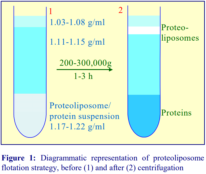 1. Background
After protein has been incorporated into some form of liposome, it is necessary to resolve the proteoliposomes from any unincorporated protein. The most widely used strategy is described in Figure 1: the sample is adjusted to a density of 1.17-1.22 g/ml by mixing with a high-density stock solution and layered beneath two lower density solutions (the top layer is sometimes the isolation buffer). During centrifugation the proteoliposomes float upwards to band at the top interface. The big advantage of this strategy is that the unincorporated protein remains in the sample zone and will even tend to sediment in the opposite direction (Figure 1). If the sample is on top of a density barrier the proteoliposomes and the free proteins sediment in the same direction; separation of the two types of particle may be less clear; such separations also require longer centrifugation times (see Section 5b).
2. Density gradient format
NycodenzⓇ was first used by Weber et al [1] and it was considered by Scott et al [2] to be “by far the best gradient medium” for separation of proteoliposomes from the unbound protein. Small scale separations comprising 300 μl of the sample in 40% (w/v) NycodenzⓇ, 250 μl of 30% NycodenzⓇ and 50 μl of buffer were run in 0.8 ml tubes for a Beckman SW55Ti rotor, centrifuged at approx. 280,000 g for 4 h. A similar format (shown in Figure 1) has been used by many workers (e.g. refs 3-6). Volumes can be increased more or less proportionately and may be as much as 2 ml, 2ml and 1 ml respectively for the SW55Ti rotor [7]. More recently the use of OptiPrep™ was introduced and it is used in a similar manner [8]. Use of OptiPrep™ is much easier and is the recommended option.
3. Solution preparation
3a. Buffer composition
In the published methods there is no consistent use a particular buffer for the gradient and it can vary from a simple buffered salt solution [8,9] or buffered sucrose solution containing 1 mM EDTA [10] to solutions containing 100 mM KCl, 10% glycerol, 1 mM DTT, 25 mM HEPES-KOH, pH 7.4 [11] or 140 mM potassium gluconate, 4 mM MgCl2, 20 mM HEPES-KOH, pH 7.3 [12]. The operator should use whatever medium is most suitable for the stability of the proteoliposomes, which may vary with the type of lipids used for the liposomes or the protein to be incorporated; for convenience simple buffered salt and sucrose solutions are given in this Application Sheet.
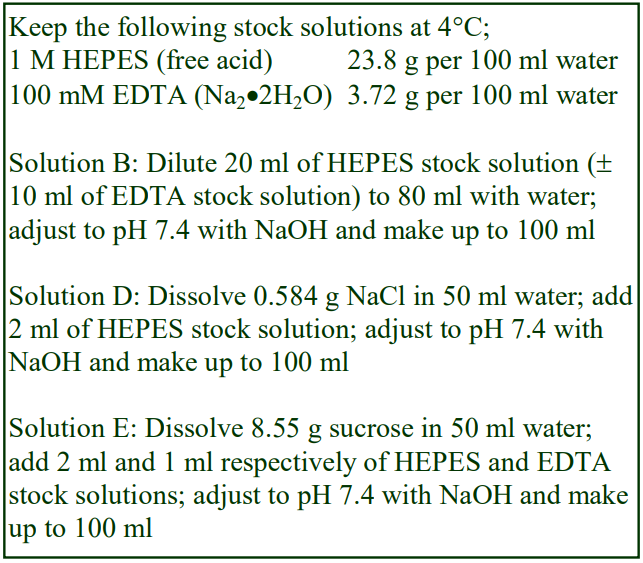 3b. Solutions required (see box on next page)
Choose either Solution D or Solution E
A. OptiPrep™ (shake the bottle gently before use)
B. OptiPrep™ diluent: 200 mM HEPES-NaOH, pH 7.4 (include 10 mM EDTA if Solution E is chosen)
C. Working solution (54% w/v iodixanol): Mix 9 vol. of OptiPrep™ with 1 vol. of Solution B
D. Liposome buffer 1: 100 mM NaCl, 20 mM HEPES-NaOH, pH 7.4
E. Liposome buffer 2: 0.25 M sucrose, 1 mM EDTA, 20 mM HEPES-NaOH, pH 7.4
Note. The preparation of the 54% (w/v) iodixanol working solutions permits the concentration of buffer, and that of the EDTA (if Solution E is chosen), to be constant in the gradient solutions and in the sample. If other reagents are considered important for the stability of the proteoliposomes, such as 1 mM DTT [11] or 4 mM MgCl2 [12], then these too may be included at 10x the required concentration in Solution B. This solution strategy avoids the 50% reduction in the concentration of these reagents if the proteoliposome suspension were simply diluted with an equal volume of neat OptiPrep. It is not normal practice to include the osmotic balancer, NaCl, KCl, sucrose or glycerol in the Working Solution. For more information on preparing gradient solutions see Application Sheet M01.
4. Ultracentrifuge rotor requirements
Swinging bucket rotors with or 0.8-5 ml tubes (e.g. Beckman SW55Ti) are commonly used. Smallvolume Beckman fixed-angle rotors have also been used with both NycodenzⓇ and iodixanol gradients: MLA130 [13], TLA100.2 [14] and TLA100.4 [9,12].
5. Gradient centrifugation
5a. Flotation in iodixanol gradients (adapted from ref 8, for variations and comments see Section 5b)
Carry out all operations at 4°C.
1. Take 2.4 vol. of the proteoliposome suspension and mix well with 3 vol. of Solution C to adjust its density to approx 1.16 g/ml.
2. Make up two solutions of 25% and 5% (w/v) iodixanol by diluting Solution C with Solution D OR E using volume ratios of 2.5:2.9 and 0.5:4.9 respectively.
3. In tubes for the chosen rotor layer the proteoliposome suspension, 25% iodixanol and 5% iodixanol solutions in using a volume ratio of approx 1.0:2.5:0.1 respectively.
4. Centrifuge at 200,000 g for 3 h. If using a fixed-angle rotor use a slow acceleration program.
5. Allow the rotor to decelerate from 2000 rpm without the brake or use a slow deceleration program if this is available on the ultracentrifuge and harvest the banded proteoliposomes from the 25%/5% iodixanol interface. The gradient may alternatively be unloaded in a series of fractions. For more information see Application Sheet M04.
5b. Other gradient options
In the protocol given in Section 5a the top layer of buffer, commonly used in NycodenzⓇ gradients, is replaced with the 5% iodixanol layer. In bottom-loaded gradients the iodixanol concentration in the proteoliposome preparation is normally either 30% (w/v) or 40% (w/v) although occasionally a lower concentration (24%) is used [15]. Variations in the gradient format are: (a) 20% and 0% [11], 24%, 18% and 3% [16]; (b) omission of the topmost layer, e.g. sample in 30% iodixanol overlaid with 18% iodixanol [9,12] and (c) sample is adjusted to approx 33% (w/v) iodixanol [17], or 30% iodixanol [18], by mixing with OptiPrep™ and overlaid with buffer. The relative volumes of sample and density layers are probably not very critical but the layer(s) above the sample should be sufficiently large enough to allow the proteoliposomes to be well separated from the unincorporated proteins.
Increased resolving power has also been reported for top-loaded 5%, 15%, 30%, 40% iodixanol gradients run in larger approx. 14 ml tube rotors run for 18 h at 150,000 g [10]. Separations have also been carried out in fixed-angle rotors at 100,000 g for 5 h [15]; while if the small-volume TLA100.4 is used only 1 h is required at 500,000 g [9,12].
6. Nucleic acid-containing liposomes
Modern strategies for the targeting of DNA nanostructures in biomedical applications have become a very active area of research. Encapsulating nucleic acids in lipid bilayer-containing structures such as exosomes or artificial polyethylene-glycolated liposomes (PEG-liposomes). Perrault, S.D. and Shih [19] used PEG-liposomes, which mimic the morphology of enveloped virus particles, provide protection against nuclease digestion and reduce immune activation. A discontinuous gradient of 28, 18, and 8% (w/v) iodixanol, layered over the crude sample in 35% iodixanol, was centrifuged for 16 h at 4°C. The gradient permitted the total removal of excess PEG-liposomes from the preparation, which floated to the top of the gradient.
7. References
1. Weber, T., Zemelman, B.V., McNew, J.A., Westermann, B., Gmachl, M., Parlati, F., Söllner, T. and Rothman, J.E. (1998) SNAREpins: minimal machinery for membrane fusion Cell, 92, 759-772
2. Scott, B.L., Vam Komen, J.S., Liu, S., Weber, T., Melia, T.J. and McNew, J.A. (2003) Liposome fusion assay to monitor intracellular membrane fusion machines Meth. Enzymol., 372, 274-300
3. Parlati, F., McNew, J.A., Fukuda, R., Miller, R., Söllner, T. and Rothman, J.E (2000) Topological restriction of SNAREdependent membrane fusion Nature, 407, 194 198
4. Koumanov, F., Jin, B., Yang, J., Holman, G.D. (2005) Insulin signaling meets vesicle traffic of GLUT4 at a plasmamembrane-activatd fusion step Cell Metab., 2, 179 189
5. Siddiqui, T.J., Vites, O., Stein, A., Heintzmann, R., Jahn, R. and Fasshauer, D. (2007) Determinants of synaptobrevin regulation in membranes Mol. Biol. Cell, 18, 2037-2046
6. Abdulreda, M.H., Bhalla, A., Chapman, E.R. and Moy, V.T. (2008) Atomic force microscope spectroscopy reveals a hemifusion intermediate during soluble N-ethylmaleimide-sensitive factor-attachment protein receptors-mediated membrane fusion Biophys. J., 94, 648-655
7. Sato, K. and Nakano, A. (2004) Reconstitution of coat protein complex II (COPII) vesicle formation from cargoreconstituted proteoliposomes reveals the potential role of GTP ahydrolysis by Sar1p in protein sorting J. Biol. Chem., 279, 1330-1335
8. Volles, M.J., Lee, S-L., Rochet, J-C., Shtilerman, M.D., Ding, T.T., Kessler, J.C. and Lansbury, P.T. (2001) Vesicle permeabilization by protofibrillar -synuclein: implications for the pathogenesis and treatment of Parkinson’s disease Biochemistry, 40, 7812-7819
9. Hu, K., Rickman, C., Carroll, J. and Davletov, B. (2004) A common mechanism for the regulation of vesicular SNAREs on phospholipid membranes Biochem. J., 377, 781-785
10. Myers, S.A., Han, J.W., Lee, Y., Firtel, R.A. and Chung, C.Y. (2005) A Dictyostelium homologue of WASP is required for polarized F-actin assembly during chemotaxis Mol. Biol. Cell, 16, 2191-2206 11. Brugger, B., Nickel, W., Weber, T., Parlati, F., McNew, J.A., Rothman, J.E. and Sollner, T. (2000) Putative fusogenic activity of NSF is restricted to a lipid mixture whose coalescence is also triggered by other factors EMBO J., 19, 1272-1278
12. Hu, K., Carroll, J., Fedorovich, S., Rickman, C., Sukhodub, A. and Davletov, B. (2002) Vesicular restriction of synaptobrevin suggests a role for calcium in membrane fusion Nature, 415, 646-650
13. Moskalenko, S., Tong, C., Rosse, C., Mirey, G., Formstecher, E., Daviet, L., Camonis, J. and White, M.A. (2003) Ra1 GTPases regulate exocyst assembly through dual subunit interactions J. Biol. Chem., 278, 51743-51748
14. Ganley, I.G. and Pfeffer, S.R. (2006) Cholesterol accumulation sequesters Rab9 and disrupts late endosome function in NPC1-deficient cells J. Biol. Chem., 281, 17890-17899
15. Moll, R.G. (2003) Protein-protein, protein-RNA and protein-lipid interactions of signal-recognition particle components in the hyperthermoacidophilic archeon Arcidianus ambivalens Biochem. J., 374, 247-254
16. Eroglu, C.A., Cronet, P., Panneels, V., Beaufils, P. and Sinning, I. (2002) Functional reconstitution of purified metatropic glutamate receptor expressed in the fly eye EMBO Rep., 3, 491-496
17. Weeke-Klimp, A.H., Bartsch, M., Morselt, H.W.M., van Veen-Hof, I., Meijer, D.K.F., Scherphof, G.L. and Kamps, J.A.A.M. (2007) Targeting of stabilized plasmid lipid particles to hepatocytes in vivo by means of coupled lactoferrin J. Drug Target., 15, 585-594
18. Perez, T.D., Nelson, W.J., Boxer, S.G. and Kam, L. (2005) E-Cadherin tethered to micropatterned supported lipid bilayers as a model for cell adhesion Langmuir, 21, 11963-11968
19. Perrault, S.D. and Shih, W.M., (2014) Virus-inspired membrane encapsulation of DNA nanostructures to achieve in vivo stability ACS Nano. 8, 5132–5140
OptiPrep™ Application Sheet M10; 9th edition, January 2020
OptiPrep™ Application Sheet M11
Analysis of protein size in pre-formed gradients
- OptiPrep™ is a 60% (w/v) solution of iodixanol in water; density = 1.32 g/ml
- To access other Application Sheets referred to in the text: return to the 2020Macroapp file and select the appropriate M-number.
1. Background
Compared to nucleic acids proteins are much less highly hydrated, consequently the water activity of the density gradient medium has rather little effect on their density. Thus in iodinated density gradient media most proteins have a density very similar to that in either CsCl or sucrose, i.e. approx 1.26 g/ml [1,2]. In metrizamide gradients proteins did not form single discrete bands; the protein profile always demonstrated a significant shoulder on the high-density side of the peak. This effect was due to a weak irreversible interaction between metrizamide and the protein molecules [1]. A similar effect is seen with the banding of proteins in NycodenzⓇ gradients, but the effect is less marked [1] suggesting that NycodenzⓇ interacts much less than metrizamide.
The density of proteins in iodixanol is similar to that in NycodenzⓇ, but there is no obvious highdensity shoulder on the protein profile, suggesting that iodixanol interacts with proteins even less than does NycodenzⓇ. However OptiPrep™ provides, for the first time, an opportunity for density banding of proteins under isoosmotic conditions (see Section 3). In all of the other commonly used media (sucrose and inorganic salts), proteins band at densities that are grossly hyperosmotic; even in
NycodenzⓇ a density of 1.26 g/ml is slightly hyperosmotic. Iodixanol solutions on the other hand can be isoosmotic up to a density of 1.32 g/ml. Although the use of an isoosmotic gradient may not have any significant benefit for protein banding, it is now recognized that a hyperosmotic environment may be deleterious to the integrity of macromolecules such as proteins. In the native state, water molecules associated with various residues on the polypeptide chain are important for maintaining its stability and their removal can lead to instability and changes in the propensity of the protein molecules to aggregate [3]. Thus iodixanol gradients are particularly important for the study of protein complex formation see Application Sheet M09.
There are also secondary advantages to the use of an iodinated density gradient medium. Because of the very low density of most nucleic acids in these media (DNA has a density of approx 1.1 g/ml in iodixanol) the study of protein-nucleic acid complexes is facilitated [1,2]. In addition, because of the inert non-ionic nature of the medium, proteins harvested from iodixanol gradients can be run on polyacrylamide gels directly without the need to remove the medium. A disadvantage of sucrose is its viscosity; protein banding thus requires long centrifugation times in this medium.
2. Use of linear NycodenzⓇ gradients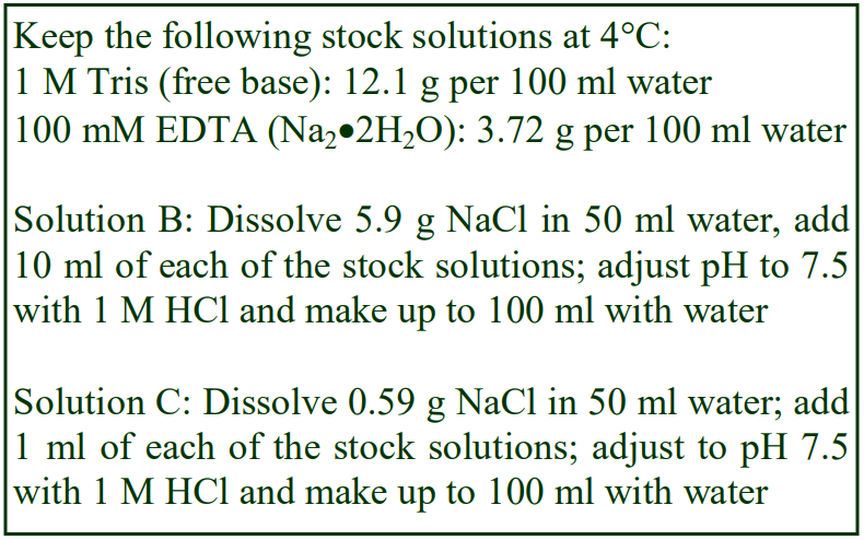
Linear NycodenzⓇ gradients have recently been reported for analysis of the oligomerization of the Ebola virus VP30 protein [4], the gradients were also very effective in the resolution of protein markers covering a wide molecular mass range.
2a. Solutions required
A. 45% (w/v) NycodenzⓇ stock solution (see Step 1 of Protocol – Section 2c)
B. NycodenzⓇ diluent: 1 M NaCl, 10 mM EDTA, 100 mM Tris-HCl, pH 7.5
C. Buffered saline: 0.1 M NaCl, 1 mM EDTA, 10 mM Tris-HCl, pH 7.5
2b. Ultracentrifuge rotor requirements
Any suitable swinging-bucket; the following protocol has been devised for the Beckman SW60Ti rotor, which accommodates 4 ml tubes (see Note 1).
2c. Protocol
1. To make up the 45% NycodenzⓇ stock solution place 50 ml of water in a 150 ml beaker on a heated magnetic stirrer set at approx. 50°C and add 45 g of powder in small amounts until dissolved. Allow the solution to cool to room temperature and then add 10 ml of Solution B and make up to 100 ml with water (see Note 2). Filter sterilize if required.
2. Make a 10% (w/v) solution of NycodenzⓇ by diluting 1 vol. of the 45% stock solution with 3.5 vol. of Solution C. iodixanol (ρ = 1.16 g/ml) by diluting OptiPrep™ with an equal volume of Solution of B.
3. Prepare a linear gradient from equal volumes of the two NycodenzⓇ solutions using a Gradient Master™ or a two chamber gradient maker or by allowing a discontinuous gradient to diffuse (see Note 3). In a 4 ml tube use a 3.6 ml gradient (see Note 4).
4. Bring the gradients to 4°C and then layer approx. 0.3 ml of the sample on top of the gradient so that the tube is filled to a level in accordance with the manufacturer’s recommendations (see Note 4).
5. Centrifuge at approx 350,000 g for approx. 22 h at 4°C (use slow acceleration and deceleration programs or turn the brake off below 3000 rpm during the deceleration).
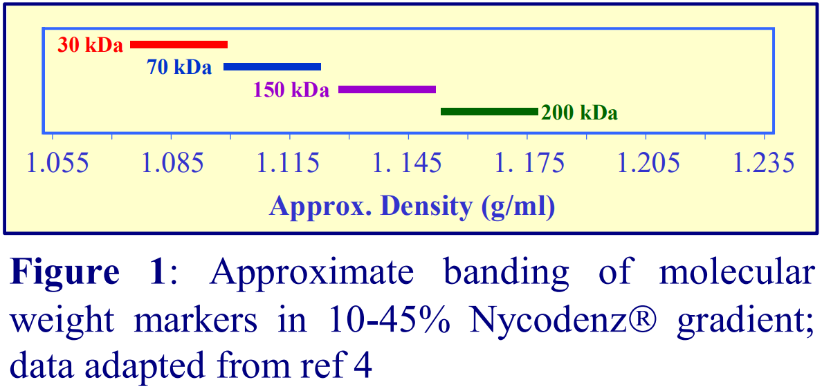 6. Collect the gradient by tube puncture or aspiration from the meniscus in approx 0.25 ml fractions (see Note 5). See Figure 1 for the approximate banding position of molecular weight markers (see Note 6).
2d. Notes
1. Other swinging-bucket rotors may be used; those with longer sedimentation path lengths will require longer centrifugation times, especially as the larger volume rotors may have a lower maximum g-force. It should be possible to adapt the method to the use of vertical rotors, in which case the centrifugation time may be considerably reduced.
2. The strategy for the preparation of the two gradient solutions, maintains the same background concentration of NaCl, EDTA and buffer throughout the gradient. If this is deemed unnecessary, the 45% (w/v) Nycodenz solution may be simply be prepared in Solution C.
3. For more detailed information on the construction of continuous gradients see Application Sheet M02.
4. The ideal volume of gradient is dictated by the need to layer the sample on the gradient in a narrow band in order to maximize the resolution of the sedimentation velocity gradient. The volume of sample should not be more than approx. 7.5% of the gradient volume.
5. For more detailed information on unloading gradients see Application Sheet M04.
6. The gradient was used very successfully by Hartlieb et al [4] to distinguish the monomeric, dimeric and hexameric forms of VP30.
3. OptiPrep™ Applications
1. Large et al [5] used a discontinuous gradient of 0.3M, 0.5M, 0.7M sucrose and 36% (w/v) iodixanol in the fractionation of CCT type II chaperonins from Haloferax volcanii.
2. Salivary mucins have been size-fractionated on 10-30% (w/v) iodixanol gradients (210,000 g for 1 h) – three types were defined based on rate of sedimentation (at approx. 1.10, 1.13 and 1.17 g/ml). The densest granular form was studied further by Kesimer et al [6].
3. Shutova et al [7] analyzed the non-muscle myosin II (NM-II)from rat embryo fibroblasts in iodixanol gradients. After cell lysis in a buffered 150 mM KCl containing 0.5% Triton-X100, lysates were centrifuged at approx. 150,000 g for 15 min to remove detergent insoluble fraction. Lysates were layered on a discontinuous gradient of 50%, 25%, 12%, and 6% (w/v) iodixanol and centrifuged at 80,000 rpm for 60 min to separate monomeric and polymerized versions of this myosin. Importantly for the use of such gradients more generally for investigating the molecular mass of proteins the authors also showed that the gradient resolved M.Wt. marker proteins aldolase, catalase and ferritin (7S, 11S and 16S respectively). The same gradient was used by Lehtimäki et al [8] to study the folding of NM-II and the assembly of bipolar filaments.
4. Vijayakumar et al [9] used an iodixanol gradient of 5-40% (w/v) centrifuged at 100,000 g for 3 h to study the oligomerization of hensin; the following markers were used to calibrate the gradient: γ-globulin (158 kDa), catalase (232 kDa), and thyroglobulin (670 kDa).
5. Linear 1-12% (w/v) iodixanol gradients were used in studies on the oligomeric state of genetically engineered fusogenic proteins on paramyxovirus replication [10].
6. Using both culture supernatants and cell lysates, after an ultrafiltration concentration step, apolipoproteins B and E from hepatitis C virus-infected cells were purified on a 10-40% (w/v) iodixanol gradient at approx 124,000 gav for 16 h [11]. Apolipoprotein(a) was shown to inhibit virus entry into hepatoma cells [12].
7. An iodixanol gradient is able to facilitate the detection of the HERV-K-ENV protein from plasma samples from individuals with an ovarian tumour or a benign tumour (or from control individuals). It was much more pronounced in the patients with ovarian tumour, while HERV-K reverse transcriptase was similarly raised in the two groups of patients [13].
4. References
1. Ford, T. and Rickwood, D. (1983) Analysis of macromolecules and their interactions In: Iodinated density gradient media – a practical approach (ed. Rickwood, D.) IRL press at Oxford University Press, Oxford, UK, pp 23-42.
2. Ford, T., Rickwood, D. and Graham, J. (1983) Buoyant densities of macromolecules, macromolecular complexes and cell organelles in Nycodenz gradients Anal. Biochem., 128, 232-239
3. Timasheff, S.N. (1993) The control of protein stability and association by weak interactions with water: How do solvents affect these processes Annu. Rev. Biophys. Biomol. Struct., 22, 67-97
4. Hartlieb, B., Muziol., T., Weissenhorn, W. and Becker, S. (2007) Crystal structure of the C-terminal domain of Ebola virus VP30 reveals a role in transcription and nucleocapsid association Proc. Natl. Acad. Sci. USA, 104, 624-629
5. Large, A.T., Kovacs, E. and Lund, P.A. (2002) Properties of the chaperonin comples from the halophilic archaeon Haloferax volcanii FEBS Lett., 532, 309-312
6. Kesimer, M., Makhov, A.M., Griffith, J.D., Verdugo, P. and Sheehan, J.K. (2010) Unpacking a gel-forming mucin: a view of MUC5B organization after granular release Am. J. Physiol. Lung Cell Mol. Physiol., 298, L15–L22
7. Shutova, M., Yang, C., Vasiliev, J.M. and Svitkina, T. (2012) Functions of nonmuscle myosin II in assembly of the cellular contractile system PLoS One, 7: e40814
8. Lehtimäki, J.I., Fenix, A.M., Kotila, T.M., Balistreri, G., Paavolainen, L., Varjosalo, M., Burnette, D.T. and Lappalainen, P. (2017) UNC-45a promotes myosin folding and stress fiber assembly J. Cell Biol., 216, 4053–4072
9. Vijayakumar, S., Peng, H. and Schwartz, G.J. (2013) Galectin-3 mediates oligomerization of secreted hensin using its carbohydrate-recognition domain.Am. J. Physiol. Renal Physiol., 305, F90–F99
10. Brindley, M.A., Plattet, P. and Plemper, R.K. (2014) Efficient replication of a paramyxovirus independent of full zippering of the fusion protein six-helix bundle domain Proc. Natl. Acad. Sci., USA, 111, E3795–E3804
11. Fukuhara, T., Wada, M., Nakamura, S., Ono, C., Shiokawa, M. et al (2014) Amphipathic -helices in apolipoproteins are crucial to the formation of infectious hepatitis C virus particles PLoS Pathog., 10, e1004534
12. Oliveira, C., Fournier, C., Descamps, V., Morel, V., Scipione, C.A., Romagnuolo, R., Koschinsky, M.L., Boullier, A., Marcelo, P. et al (2017) Apolipoprotein(a) inhibits hepatitis C virus entry through interaction with infectious particles Hepatology, 65, 1851-1864
13. Rycaj, K., Plummer, J.B., Yin, B., Li, M., Garza, J., Radvanyi, L., Ramondetta, L.M. et al (2015) Cytotoxicity of human endogenous retrovirus K–specific T cells toward autologous ovarian cancer cells Clin. Cancer Res., 21, 471–83
OptiPrep™ Application Sheet M11; 9th edition, January 2020
OptiPrep™ Application Sheet M12
Analysis of proteins in small volume self-generated gradients
- OptiPrep™ is a 60% (w/v) solution of iodixanol in water, density = 1.32 g/ml
- To access other Application Sheets referred to in the text: return to the 2020Macroapp file and select the appropriate M-number.
- For more background information on the use of iodinated density gradient media for protein analysis see the companion Application Sheet M11
1. Background
Continuous sucrose gradients in swinging-bucket rotors are still used for the fractionation of proteins on the basis of sedimentation rate. Continuous gradients are generated by diffusion of discontinuous gradients or by a gradient making device. Centrifugation times are usually at least 4 h and may be as long as 16 h and if, as is often the case, these gradients are used for analyzing the formation of protein-protein and protein-nucleic acid complexes, these macromolecular complexes may be insufficiently stable to survive these long times. The stability of protein complexes is also affected by the hydrostatic pressure that is generated in a gradient [1,2] and in a standard swinging-bucket rotor this pressure can be considerable. Basi and Rebois [3] adapted these procedures to the use of OptiPrep™ in small volume (200 µl) self-generated gradients.
The strategy is to centrifuge a uniform concentration of iodixanol at approx 350,000 g to form a self-generated gradient; then to layer the proteins on top of the gradient and recentrifuge for no more than 1 h. Thick-walled open-topped polycarbonate tubes must be used to allow these operations. Such small volume tubes pose a problem for the subsequent harvesting and must be carried out low-density end first using a Brandel Microfractionator™ or a Labconco Auto Densi-flow™. T
he molecular mass of membrane proteins solublized in either dodecyl-maltoside or octylglucoside has been analyzed by analytical ultracentrifugation, using dense NycodenzⓇ stock solutions for density adjustment in sedimentation velocity and sedimentation equilibrium runs. For more details
of this specialized methodology see ref 4.
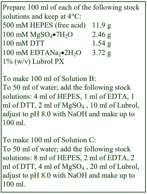 2. Solutions required
A. OptiPrep™
B. Protein solution: 20 mM HEPES-NaOH, pH 8.0, 1 mM EDTA, 1 mM dithiothreitol, 2 mM MgSO4 and 0.1% Lubrol PX.
C. Diluent: 40 mM HEPES-NaOH, pH 8.0, 2 mM EDTA, 2 mM dithiothreitol, 4 mM MgSO4 and 0.2% Lubrol PX (see Note 1).
D. Protein solution (1.0-1.2 mg/ml)
3. Ultracentrifuge rotor requirements
Beckman TLA100, TLA 100.1 or TLA120.1, Sorvall S100-AT3, RP100-AT3, S120-AT3. Larger volume rotors such as the Beckman TLA100.2 or Sorvall S150-AT may be suitable (see Note 2).
Only open-topped tubes are suitable for this application, sealed tubes cannot be re-sealed once they have been centrifuged. Moreover such tubes cannot be easily unloaded low-density end first.
4. Protocol
1. Mix equal volumes of OptiPrep™ and Solution C to produce a 30% (w/v) iodixanol working solution. This can either be used directly as the gradient forming solution or diluted further with Solution B as required.
2. Fill a thick-walled open-topped centrifuge to the recommended level with 30%.
3. Centrifuge at 350,000 gav for 2-3 h to self-generate the gradient (see Note 3).
4. Allow the rotor to decelerate from 2000 rpm using a controlled deceleration program to allow a smooth reorientation of the gradient.
5. Layer a small volume (10 µl on top of a 0.2 ml gradient; 50 µl on top of a 2.0 ml gradient).
6. Recentrifuge the gradients at approx 250,000 gav for approx 1 h (see Note 4). Use controlled programs for acceleration to and deceleration form 2000 rpm.
7. Collect the gradient using a Brandel Microfractionator or some other appropriate system (see Note 5).
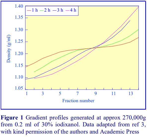 5. Notes
1. The protein solution and diluent can contain any low concentrations of reagents that will aid protein stability without materially affecting their density. Some glycoproteins may need slightly higher starting concentrations of iodixanol. For more information about the preparation of gradient solutions see Application Sheet M01.
2. Basi and Rebois [3] used an adapted Beckman TLA 120.2 rotor to reduce the tube volume to 0.2 ml, but there are many other standard Beckman and Sorvall rotors (see Ultracentrifuge rotor requirements) that accommodate similar volumes and will produce linear gradient profiles of the type shown in Figure 1 (2/3h). Larger volume rotors are also capable of producing approximately linear gradients at higher RCFs. For more information on the formation of self-generated gradients see Application Sheet M03.
3. The centrifugation conditions required to produce a suitable density gradient profile will vary with rotor type (see Note 2 for linked files).
4. The centrifugation conditions required will vary with the sedimentation path length of the rotor and the size of the proteins. Figure 2 and Note 6 summarize some of the data obtained by Basi and Rebois [3]. Some experimentation may be required to optimize the system to suit the operator’s requirements.
5. To fractionate these small volume (<0.5 ml) gradients, Basi and Rebois [3] used a Brandel Automated Microfractionator. This device uses a fine stepper motor to advance a metal cylinder into the centrifuge tube (in 0.35 mm steps). The gradient is displaced up through a central channel in the cylinder. At the top of the cylinder a T-piece allows successive equivolume fractions to be expelled into the collection tubes. It can provide fractions of as little as 6 µl. With larger volume gradients (approx 2 ml) it may be possible to collect from the bottom of the gradient using narrow bore tubing connected to peristaltic pump. For more information on harvesting gradients see Application Sheet M04.
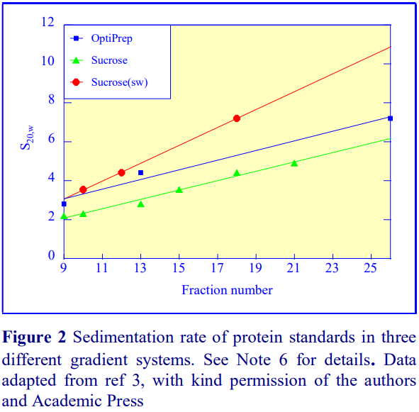 6. Figure 2 shows the sedimenting characteristics in iodixanol gradients of some standard proteins (lysozyme, soya bean trypsin inhibitor, carbonic
anhydrase, ovalbumin, bovine serum albumin, transferrin and -globulin). The sedimentation coefficient of these proteins is plotted against the fraction number to obtain a straight-line graph. Three types of gradient are compared: (a) a 2 h self-generated gradient of iodixanol, recentrifuged after sample loading at 100,000
rpm for 1 h; (b) a pre-formed 5-20% (w/v) sucrose gradient (formed by diffusion of a discontinuous gradient), in the same tubes, centrifuged at 120,000 rpm for 1 h and (c) a preformed 5-20% sucrose gradient run in a standard swinging-bucket rotor (Beckman SW50.1) and centrifuged at 43,000 rpm for 17 h.
6. References
1. Marcum, J. M. and Borisy, G. G. (1978) Sedimentation velocity analyses of the effect of hydrostatic pressure on the 30 S microtubule protein oligomer J. Biol. Chem., 253, 2852-2857
2. Hauge, J. G. (1971) Pressure induced dissociation of ribosomes during ultracentrifugation FEBS Lett., 17, 168-172
3. Basi, N.S. and Rebois, V. (1997) Rate zonal sedimentation of proteins in one hour or less Anal. Biochem., 251, 103-109
4. Lustig, A., Engel, A., Tsiotis, G., Landau, E.M. and Baschong, W. (2000) Molecular weight determination of membrane proteins by sedimentation equilibrium at the sucrose or Nycodenz-adjusted density of the hydrated detergent micelle Biochim. Biophys. Acta, 1464, 199-206
7. Acknowledgements
We wish to thank Dr R Victor Rebois, Membrane Biochemistry Section, NINDS, NIH, Bethesda, MD 20892, USA for his cooperation in the preparation of this manuscript.
OptiPrep™ Application Sheet M12; 7th edition, January 2020
OptiPrep™ Application Sheet M13
Fractionation of nucleic acids and nucleic acid-protein complexes
- OptiPrep™ is a 60% (w/v) solution of iodixanol in water; density = 1.32 g/ml
- To access other Application Sheets referred to in the text: return to the 2020Macroapp file and select the appropriate M-number.
1. Introduction
Sucrose sedimentation velocity gradients are widely used in the analysis of polysomes and their component ribosomal subunits, of messenger ribonucleoproteins (mRNPs) and of the nuclear heterogeneous ribonucleoproteins (hnRNP). Separation of mRNP from ribosomal subunits is however difficult by this method. An alternative is to fractionate the particles according to density, but to provide the necessary high density it has been necessary to use heavy metal salts (e.g. CsCl). Such high ionic strength gradients however have serious shortcomings and to prevent dissociation of the macromolecular components particles are fixed in formaldehyde or glutaraldehyde. Ford and Rickwood [1] and Houssais [2] developed the use of gradients of the non-ionic gradient solute NycodenzⓇ. Not only is it unnecessary to prior fix the particles, the high water activity (low osmolality) of NycodenzⓇ solutions compared to those of CsCl means that the RNA molecules retain their normal levels of hydration. Ford and Rickwood [1] showed that in NycodenzⓇ 40 molecules of water were bound to each mole of nucleotide, while in CsCl this figure dropped to 3. Consequently the density of RNA in NycodenzⓇ is much lower than that in CsCl, 1.184 g/ml against >1.9 g/ml. NycodenzⓇ gradients therefore offer great advantages over those of CsCl and other heavy metal salts.
It is likely (but untested) that iodixanol could substitute for Nycodenz and since iodixanol solutions are prepared much more easily from OptiPrep™, some suggestions are given in Section 3. Published OptiPrep™-based methods primarily on DNA- and RNA-complexes are given in Section 4.
2. NycodenzⓇ-based methodology
2.1 Gradient solution preparation
NycodenzⓇ gradients have been used for the analysis of RNA-containing complexes from Xenopus oocytes or embryos and from mammalian cells. In both cases the gradients cover a broad range of densities, commonly from approx 1.05 or 1.10 g/ml to 1.32 g/ml (equivalent to 10-20% NycodenzⓇ to 60% (w/v) NycodenzⓇ).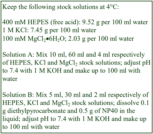
Xenopus
Tafuri and Wolffe [3] used a 20-60% (w/v) NycodenzⓇ gradient containing 0.3 M KCl, 2 mM MgCl2, 20 mM HEPES, pH 7.4 containing 0.1% diethylpyrocarbonate and 0.5% NP40 To make up a stock solution of 60% (w/v) NycodenzⓇ place 50 ml of Solution A (see box) in a 150 ml beaker on a heated magnetic stirrer set at approx.
50°C and add 60 g of NycodenzⓇ powder in small amounts until dissolved. Allow the solution to cool to room temperature, dissolve 0.1 g diethylpyrocarbonate and 0.5 g of NP40 and make up to 100 ml with water.
Filter sterilize if required. Make up solutions of lower density by dilution of the 60% NycodenzⓇ stock
with Solution B. This strategy for making up the gradient solutions maintains the concentrations of
Excellence in Separations
Mammalian cells and tissues
The solutions used for the gradient reflect the different solutions selected for homogenizing the cells. NycodenzⓇ solutions for analyzing cytoplasmic extracts have been prepared in the following: 150 mM KCl, 3 mM MgCl2, 50 mM Tris-HCl, pH 7.6 containing 1 mM DTT, together with protease inhibitors and rRNasin [4] or 115 mM KCl, 20 mM HEPES-KOH, pH 7.3 [5], while for nuclear extracts Ladomery et al [6] used 2mM MgCl2, 1 mM EDTA, 20 mM Tris-HCl, pH 7.5.
The same principles regarding solution preparation apply as described in section 2a. If it is important that the reagent concentration should be constant in the gradient make up the 60% (w/v) NycodenzⓇ solution initially using double concentration buffer to dissolve the NycodenzⓇ or if this is not important use the regular buffer for all solution preparation.
2.2. Ultracentrifuge rotor requirements
In most cases a 4-5 ml gradient is used, so Beckman rotors such as the SW55Ti or SW50.1, or Sorvall rotors such as the AH650 or TH660 are suitable. Sometimes the gradient volume is smaller, e.g. a 1.5 ml gradient in a Beckman TLS-55 [3].
2.3. Gradient preparation
Gradients for Xenopus material are usually 20-60% (w/v) NycodenzⓇ [3,7] for cultured mammalian cells 10-60% [4,5,8,9] or 20-60% [6,10,11]. For mouse testis 20-60% is the chosen gradient type [12,13] Sample volumes are routinely small (approx. 0.2 ml, but may be as large as 1 ml) so the total gradient volume needs to be adjusted accordingly to take account of the sample load so that the tubes are filled according to the manufacturer’s instructions. Prepare continuous gradients from equal volumes of the densest and lightest solution in either a two-chamber gradient maker or a Gradient Master™. Alternatively prepare a discontinuous gradient from equal volumes of e.g. 10%, 22.5%, 35%, 47.5% and 60% (w/v) NycodenzⓇ and allow to diffuse for 3-4 h at room temperature. Bring all gradients to 4°C before use. For more information on making these gradients see Application Sheet M02.
2.4. Sample loading and centrifugation
Carry out all operations on at 4°C. Centrifuge the cell lysate at approx. 800 g for 8 min; the 800 g supernatant at 12-15,000 g and then load this supernatant on to the gradient. The most commonly used centrifugation condition for the gradient is 150,000 g for 16-22 h at 4°C, although 44 h at 75,000 g has also bee reported [4,8]. Allow the rotor to decelerate from 3000 rpm without the brake or use a slow deceleration program.
2.5. Gradient harvesting
The gradients are routinely harvested in small equal volume fractions (approx 75-125 μl). Lowdensity end first is recommended because of the viscosity of the densest fractions. Upward displacement with a dense medium or aspiration from the meniscus are recommended. For more information on unloading gradients see Application Sheet M04.
2.6. Analysis
Analysis of the fractions from Xenopus oocytes showed that 42S RNPs (distinguished by the presence of 4-5S RNA) banded in the top third of the gradient; RNPs containing mRNA in the middle third and ribosomes in the bottom third [3]. Mammalian cells demonstrated a similar distribution; free proteins were observed in fractions 4-10, overlapping the 5S RNA, mRNPs banded in the middle (fractions 14-17) and polysomes in fractions 18-23 [10]. The gradient was used to show that an IGF-IImRNA binding protein localizes not to the endoplasmic reticulum, which banded around 1.09-1.16 g/ml but to RNPs around 1.23 g/ml [5]. Fractionation of material from mouse testis revealed that the majority of the mRNA was associated with non-polysomal mRNP fractions, distinct from monosomes and polysomes [12]. Nuclear extracts analyzed on these (and metrizamide gradients) showed that cytoplasmic messenger RNP peaked around 1.21 g/ml while pre-mRNP banded around 1.31 g/ml and at 1.18 g/ml [14].
3. Using OptiPrep™ as a replacement for NycodenzⓇ
There is no obvious reason why iodixanol cannot be substituted for NycodenzⓇ. Its availability as a sterile 60% (w/v) solution (OptiPrep™) generally makes solution preparation much more easy (see Application Sheet M01), the most convenient way of preparing solutions containing 0.3 M KCl, 2 mM MgCl2, 20 mM HEPES-KOH, pH 7.4 would be to dilute 5 vol. of OptiPrep™ with 1 vol. of 1.8 M KCl, 12 mM MgCl2, 120 mM HEPES-KOH, pH 7.4, so the highest achievable iodixanol concentration would be 50% (w/v).
4 OptiPrep™-based methods
4.1 Ribonucleoproteins
Apcher et al [15] studied the capacity of the glycine-alanine repeat (GAr) sequence of the EpsteinBarr virus-encoded EBNA-1 to suppress mRNA translation in cis. Iodixanol gradients (not defined) centrifuged at 155,000 g for 2 h, were able to identify 40S ribosomes, 60S ribosomes and 80S ribosomes + polysomes. See also Section 4.7.
4.2 Hepatitis C virus RNA
Hepatitis C virus (HCV) released from infected human hepatoma cells has been analyzed in iodixanol gradients. The RNA-containing material was first concentrated on a cushion of 40% (w/v) iodixanol in Tris-buffered 0.85% NaCl at 52,000 g for 6 h. After discarding the supernatant the interfacial material was mixed into the cushion; overlaid by a 0-28% iodixanol gradient and centrifuged at 110,000 g for 16 h. The characteristic lipid rich RNA containing particles banded at 1.04-1/06 g/ml, while residual RNA banded at 1.13 g/ml [16]. A broadly similar dichotomy of low density lipidassociated RNA and high density RNA from HCV-infected cells has been observed using selfgenerated iodixanol gradients [17-21]. In this case the cell homogenate was simply adjusted to approx. 25% (w/v) iodixanol, 0.084 M sucrose, 4.8 mM EDTA, 20 mM Tris-HCl, pH 7.4 and centrifuged at 165,000 g for 24 h.
4.3 Hepatitis B nucleocapsid
Wang et al [22] analyzed DDX3, HBV Pol, and the core protein from lysed transfected HEK293 cells in 2 ml 10-50% (w/v) iodixanol gradients in 1% NP-40, 150 mM NaCl, 1 mM EDTA, 50 mM Tris-HCl, pH 7.4 (plus protease inhibitors); the gradients were centrifuged at approx. 200,000 gav for 45 min at 20°C. Each protein had a distinct density distribution profile and the DDX3 protein was shifter to lower densities after RNase A treatment and the iodixanol gradient showed that it is this protein that is incorporated into nucleocapsids.
Kim et al [23] also used small volume sedimentation velocity gradients of the same range, again made up by dilution of OptiPrep™ with cell lysis buffer and centrifuged under the same conditions. The gradient showed that unlike wild-type Pol, mutant Pols were not incorporated into capsid particles. This gradient demonstrated that core proteins of the nucleocapsid banded about two-thirds of the way down the gradient, Pol on the other hand, while overlapping the core proteins, showed a broader distribution towards lower densities [23]. The eIF4E (a eukaryotic translation initiation factor) showed a biphasic distribution, predominating in the lower density fractions (maybe polysomes). Proteinase K and RNase treatment caused a loss of the less dense banding of both eIF4E and Pol, which were detected only in the denser nucleocpasid region of the gradient [24].
4.4 Micro RNA
Detzer et al [25] analyzed siRNA and RNAi-associated proteins from normal and NaAsO2-stressed ECV 304 cells; post-nuclear supernatants were layered on top of 10-25% (w/v) iodixanol gradients in 250mM sucrose, 140mM NaCl, 1mM EDTA, 20mM Tris–HCl, pH 8.0, 2mM DTT and centrifuged at 48,000 g for 18 h.
4.5 Mitochondrial nucleic acids and nucleoproteins
He et al [26] and Di Re et al [27] described the use of iodixanol gradients for the analysis of mitochondrial nucleoproteins. A hypotonic DDM-containing medium was used to lyse trypsinized mitochondria; then after a low-speed centrifugation (1000 g for 10 min) the lysate was loaded on to a 20–45% (w/v) iodixanol gradient (in 20 mM HEPES-NaOH pH 7.6, 1mM EDTA, 25mM NaCl, 1mM DTT, 0.1% DDM) and centrifuged at 100,000 g for 12 h. For more details see refs 26 and 27. The mtDNA bands sharply in the gradient at approx. 30-32.5% (w/v) iodixanol and it binds proteins involved in mitochondrial nucleoid organization [26] and DNA polymerase γ (POLGβ) [27]. More recently the same group has reported the binding of -actin, myosin and TFAM [28]
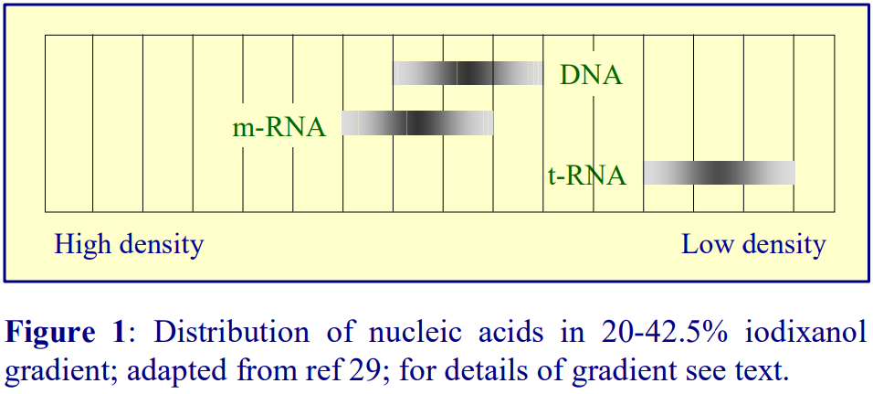 A slightly shallower gradient of 20–42.5% (w/v) iodixanol gradient run for 14 h was used by Sharma et al [29]. The distribution of tRNA, m-RNA and DNA in the gradient is shown diagrammatically in Figure 1. This gradient showed that mtDNA associated with (a) the telomerase reverse transcriptase [29] (b) PABPC5 (a member of the cytosolic poly(A) binding protein family) [30], (c) recombinant C4orf14 [31]. In spite of the proximity of m-RNA and mtDNA in the gradient the careful fractionation used by He et al [32] in their studies on nucleoid interacting proteins and mitochondrial protein synthesis, clearly demonstrated that some proteins were primarily bound to m-RNA and others to mtDNA. Kazak et al [33] showed that an isoform of replication protein Flap endonuclease 1 interacts with RNA/DNA hybrids in mtDNA.
A gradient of 10-50% (w/v) iodixanol centrifuged at 85,000 g for 15 h was used in studies of the involvement of specific m-RNAs in circadian clock negative feedback [34].
Detergent-solubilized mitochondria from HEK cells, when analyzed by a top-loaded 20-42.5% (w/v) iodixanol gradient (100,000 g for 14h) showed that PrimPol, a DNA primase and polymerase, was resolved from mtDNA and DNA maintenance proteins. However formaldehyde cross-linking prior
to detergent lysis revealed a transient cross-linking of PrimPol with mtDNA [35]. Identical gradient and centrifugation conditions were used by Rosa et al [36] to show that the protein MPV171.2 cofractionated with mitochondrial nucleoids.
A similar gradient, in which the sample was bottom-loaded was used by Rajala et al [37] to study the association of replication factors with mtDNA. Briefly, purified mitochondria were either lysed in Triton X-100 with or without a preliminary pelleting of the membranes with digitonin. The material was adjusted to 42.5% (w/v) iodixanol and overlaid with a discontinuous 0, 20% and 25-40% iodixanol gradient (in 2.5% steps), containing buffered saline and 1% T-X100. The mtDNA + nucleoid-associated protein banded at approx 25-27% iodixanol, while larger ribosomal subunit proteins banded at approx. 37.5% iodixanol after centrifugation at 100,000 g for 14 h.
Studies of mtDNA nucleoids by Lee et al [38] and Bogenhagen [39] use a double gradient approach which used a sedimentation velocity glycerol gradient followed by a buoyant density iodixanol gradient. Briefly, mitochondria were lysed in Triton X100 and the clarified material was loaded on to a 15-40% glycerol gradient (over a cushion of 30% (w/v) iodixanol/20% glycerol) and centrifuged at 210,000 g for 4 h. The nucleoids (which banded close to the bottom of the gradient) and the mitochondrial ribosomes (peak banding approx. 23% glycerol) were harvested and re-run through a 20-40% (w/v) iodixanol gradient, centrifuged at 140,000 g for 12-14 h. In this gradient mtDNA and the DNA-binding protein (TFAM) banded around 33% iodixanol, while ribosomal complexes banded at High density Low density t-RNA DNA m-RNA approx 26% iodixanol. A detailed account of the double-gradient procedures for resolution of these mitochondrial nucleoids can be found in ref 40.
Gerhold et al [41] used a flotation strategy to show that the helicase Twinkle, which is required for mtDNA replication in nucleoids is associated with a detergent-resistant membrane domain that was resolved by floatation through an iodixanol gradient. The discontinuous gradient, which was formed from 40, 37.5, 35, 32.5, 30, 27.5, 25, 20 and 0% iodixanol solutions containing 1% Triton X-100 was under-layered by the detergent-treated membrane sample and centrifuged at 100000 g for 14 h. During the centrifugation the gradient would have become continuous; Twinkle and DNA co-banded towards the top of the gradient.
4.6. Analysis of Tacaribe virus nucleoproteins
In a study of RNA replication in Tacaribe virus Baird et al [42] developed a very useful iodixanol gradient for the analysis of replication transcription complexes (RTCs). The virus-containing cells are lysed in a medium containing K-aspartate, K-glutamate and K-gluconate (all 38 mM), !0 mM KHCO3, 2 mM MgCl2 (or 5 mM EDTA), 2mM DTT, 10M ZnCl2 and 20 mM MOPS pH 7.1 (plus protease inhibitors), either by Dounce homogenization or addition of a detergent (2% NP40). A 15-48% (w/v) iodixanol gradient (containing the same reagents as the lysis medium) is formed in 5 ml tubes for a swinging-bucket rotor; either using a gradient former or by allowing a discontinuous gradient (equal volumes of 15%, 26%, 37% and 48% iodixanol to diffuse. After adjusting the sample to 50% (w/v) iodixanol it is layered beneath the continuous gradient and centrifuged at 100,000 g for 20 h. For more information on gradient formation and the underlayering of samples see Application Sheet M02. As with all flotation gradients, soluble proteins remain in the load zone, allowing the other macromolecules and macromolecular complexes to float into the gradient. Most of the Tacaribe virus nucleoprotein banded at a density that confirmed its association with the virus membrane [42]. Importantly the gradient was also able to distinguish the full length RNAs (which co-banded with the nucleoprotein) and denser mRNA nucleoprotein. Baird et al [42] also observed that the gradient was able to resolve other novel RNA species. For more information on the analysis see ref 42.
4.7 RNA granules
Fritzsche et al [43] designed a gradient system to purify the neuronal granules that transport RNAs to dendrites. A soluble fraction (20,000 g/15 min supernatant) was layered over a 15-30% iodixanol gradient and centrifuged at 280,000 g for 2 h. The granules banded in the middle of the gradient and were well separated from the soluble proteins, which remained near the top of the gradient. This methodology was also used by Donlin-Asp et al [44] for the study of fibroblastic ribonucleoproteins from patients with spinal muscular atrophy [44].
4.8 siRNA carriers
Separation of excess nanogel surfactant from the surfactant-coated siRNA was achieved by sedimenting the particles through 7.5% OptiPrep at 30,000 g for 30 min [45].
4.9 Separation of ribosomsal and non-ribosomal RNA
In a study of the stress complexes from kidney proximal tubule cells, the cell extract (adjusted to 2.5% iodixanol) was analyzed on a gradient of 5, 10, 15, 20, 25, 50 and 54% iodixanol (155,000 gav for 3 h). Cytoplasmic proteins were found at the top of the gradient, non-ribosomal RNA in the 2.5-15%, while ribosomal RNA banded in the 20-54% region [46].
4.10 DNA nanotechnology
New methods of encapsulating DNA may use iodixanol gradients for purification (see refs 47-49).
5. References
1. Ford, T. and Rickwood, D. (1983) Analysis of macromolecules and macromolecular interactions using isopycnic centrifguation In Iodinated density gradient media – a practical approach (ed Rickwood D.) Oxford University Press, Oxford, UK, pp 23-42
2. Houssais, J.F. (1983) Fractionation of ribonucleoproteins from eukaryotes and prokaryotes. In Iodinated density gradient media – a practical approach (ed Rickwood D.) Oxford University Press, Oxford, UK, pp 43-67
3. Tafuri, S.R. and Wolffe, A.P. (1993) Selective recruitment of masked maternal mRNA from messenger ribonucleoprotein particles containing FRGY2 (mRNP4) J. Biol. Chem., 268, 24255-24261
4. Antic, D. and Keene, J.D (1998) Messenger ribonucleoprotein complexes containing human ELAV proteins: interactions with cytoskeleton and translational apparatus J. Cell Sci., 111, 183-197
5. Nielsen, F.C., Nielsen, J., Kristensen, M.A., Koch, G. and Christiansen, J. (2002) Cytoplasmic trafficking of IGF-II mRNA-binding protein by conversed KH domains J. Cell Sci., 115, 2087-2097
6. Ladomery, M., Sommerville, J., Woolner, S., Slight, J. and Hastie, N. (2003) Expression in Xenopus oocytes shows that WT1 binds transcripts in vivo, with a central role for zinc finger one J. Cell Sci., 116, 1539-1549
7. Han, S-Y., Xie, W., Hammes, S.R. and DeJong, J. (2003) Expression of the germ cell-specific transcription factor ALF in Xenopus oocytes compensates for translational inactivation of the somatic factor TFIIA J. Biol. Chem., 278, 45586-45593
8. Keene, J.D. (2001) Ribonucleoprotein infrastructure regulating the flow of genetic information between the genome and the proteome Proc. Natl. Acad. Sci. USA, 98, 7018-702443
9. Jønson, L., Vikesaa, J., Krogh, A., Nielsen, L.K., Hansen, T.O., Borup, R., Johnsen, A.H., Christiansen, J. and Nielsen, F.C. (2007) Molecular composition of IMP1 ribonucleoprotein granules Mol. Cell. Proteomics, 6, 798-811
10. Stenina, O.I., Shaneyfelt, K.M. and DiCorleto, P.E. (2001) Thrombin induces the release of the Y-box protein dbpB from mRNA: a mechanism of transcriptional activation Proc. Natl. Acad. Sci. USA, 98, 7277-7282
11. Morrison, A.A., Viney, R.L. and Ladomery, M.R. (2008) The post-transcriptional roles of WT1, a multifunctional zincfinger protein Biochim. Biophys. Acta, 1785, 55-62
12. Tafuri, S.R., Familari, M. and Wolffe, A.P. (1993) A mouse Y box protein, MSY1, is associated with paternal mRNA in spermatocytes J. Biol. Chem., 268, 12213-12220
13. Herbert, T.P. and Hecht, N.B. (1999) The mouse Y-box protein, MSY2, is associated with a kinase on non-polysomal mouse testicular mRNAs Nucleic Acid. Res., 27, 1747-1753
14. Ladomery, M.R., Slight, J., Mc Ghee, S. and Hastie, N.D. (1999) Presence of WT1, the Wilm’s tumor suppressor gene product, in nuclear Poly(A)+ ribonucleoprotein J. Biol. Chem., 274, 36520-36526
15. Apcher, S., Komarova, A., Daskalogianni, C., Yin, Y., Malbert-Colas, L. and Fåhraeus, R. (2009) mRNA translation regulation by the Gly-Ala repeat of Epstein-Barr virus nuclear antigen 1 J. Virol., 83, 1289-1298
16. Pietschmann, T., Lohmann, V., Kaul, A., Kreiger, N., Rinck, G., Rutter, G., Strand, D. and Bartenschlager, R. (2002) Persistent and transient replication of full-length hepatitis C virus genomes in cell culture J. Virol., 76, 4008-4021
17. Nielsen, S., Pumeechockchai, W. and Burt, A. (2002) Characterization of HCV RNA particles from the serum of a patient with common variable immunodeficiency on isotonic iodixanol (OptiPrep) gradients. Association with apolipoprotein-B100 J. Hepatol., 36, Suppl. 1, 87
18. Nielsen, S., Bassendine, M., Burt, A. and Toms, G. (2002) Characterization of the structural proteins of HCV isolated from human liver J. Hepatol., 36, Suppl. 1, 87
19. Nielsen, S., Bassendine, M.F., Burt, A. and Toms, G.L. (2003) Characterization of the genome and structural proteins of -lipoprotein associated HCV extracted from infected human liver GUT, Br. Associat. Study of Liver Meeting 2002, abstr. 94
20. Nielsen, S., Bassendine, M., Neely, D., Ibrahim, S. and Toms, G. (2007) Characterization of hepatitis C virus associated with very low density lipoprotein (VLDL) in infected human serum and liver Atherosclerosis, 194, 284
21. Martin, C., Nielsen, S.U., Ibrahim, S., Bassendine, M.F. and Toms, G.L. (2008) Binding of liver derived low density hepatitis C virus to human hepatoma cells J. Med. Virol., 80, 816-823
22. Wang, H., Kim, S. and Ryu, W-S. (2009) DDX3 DEAD-box RNA helicase inhibits hepatitis B virus reverse transcription by incorporation into nucleocapsids J. Virol., 83, 5815-5824
23. Kim, S., Lee, J. and Ryu, W-S. (2009) Four conserved cysteine residues of the Hepatitis B virus polymerase are critical for RNA pregenome encapsidation J. Virol., 83, 8032-8040
24. Kim, S., Wang, H. and Ryu, W-S. (2010) Incorporation of eukaryotic translation initiation factor eIF4E into viral nucleocapsids via interaction with hepatitis B virus polymerase J. Virol., 84, 52-58
25. Detzer, A., Engel, C., Wünsche, W. and Sczakiel, G. (2011) Cell stress is related to re-localization of Argonaute 2 and to decreased RNA interference in human cells Nucleic Acids Res., 39, 2727–2741
26. He, J., Mao, C-C., Reyes, A., Sembongi, H., Di Re, M., Granycome, C., Clippingdale, A.B., Fearnley, I.M., Harbour, M., Robinson, A.J., Reichelt, S., Spelbrink, J.N., Wlaker, J.E. and Holt, I.J. (2007) The AAA+ protein ATAD3 has displacement loop binding properties and is involved in mitochondrial nucleoid organization J. Cell Biol., 176, 141-146
27. Di Re, M., Sembongi, H., He, J., Reyes, A., Yasukawa, T., Martinsson, P., Bailey, L.J., Goffart, S., Boyd-Kirkup, J.D., Wong, T.S., Fersht, A.R., Spelbrink, J.N. and Holt, I.J. (2009) The accessory subunit of mitochondrial DNA polymerase c determines the DNA content of mitochondrial nucleoids in human cultured cells Nucleic Acids Res., 37, 5701–5713
28. Reyes, A., He, J., Mao, C.C., Bailey, L.J., Di Re, M., Sembongi, H., Kazak, L., Dzionek, K., Holmes, J.B., Cluett, T.J., Harbour, M.E., Fearnley, I.M., Crouch, R.J., Conti, M.A., Adelstein, R.S., Walker, J.E. and Holt, I.J. (2011) Actin and myosin contribute to mammalian mitochondrial DNA maintenance Nucleic Acids Res., 39, 5098-5108
29. Sharma, N.K., Reyes, A., Green, P., Caron, M.J., Bonini, M.G., Gordon, D.M., Holt, I.J. Hertzog Santos, J. (2012) Human telomerase acts as a hTR-independent reverse transcriptase in mitochondria Nucleic Acids Res. 40, 712-725
30. Kazak, L., Reyes, A., Duncan, A.L., Rorbach, J., Wood, S.R., Brea-Calvo, G., Gammage, P.A., Robinson, A.J., Minczuk, AM. and Holt, I.J. (2013) Alternative translation initiation augments the human mitochondrial proteome Nucleic Acids Res., 41, 2354–2369
31. He, J., Cooper, H.M., Reyes, A., Di Re, M., Kazak, L., Wood, S.R., Mao, C.C., Fearnley, I.M., Walker, J.E. and Holt, I.J. (2012) Human C4orf14 interacts with the mitochondrial nucleoid and is involved in the biogenesis of the small mitochondrial ribosomal subunit Nucleic Acids Res., 40, 6097–6108
32. He, J., Cooper, H.M., Reyes, A., Di Re, M., Sembongi, H., Litwin, T.R., Gao, J., Neuman, K.C., Fearnley, I.M., Spinazzola, A., Walker, J.E. and Holt, I.J. (2012) Mitochondrial nucleoid interacting proteins support mitochondrial protein synthesis Nucleic Acids Res., 40, 6109–6121
33. Kazak, L., Reyes, A., He, J., Wood, S.R., Brea-Calvo, G., Holen, T.T. and Holt, I.J. (2013) A cryptic targeting signal creates a mitochondrial FEN1 isoform with tailed R-loop binding poperties PLoS One, 8: e62340
34. Padmanabhan, K., Robles, M.S., Westerling, T. and Weitz, C.J. (2012) Feedback regulation of transcriptional termination by the mammalian circadian clock PERIOD complex Science, 337, 599-602
35. García-Gómez, S., Reyes, A., Martínez-Jiménez, M.I., Chocrón, E.S., Mourón, S., Terrados, G., Powell, C., Salido, E., Méndez, J., Holt, I.J. and Blanco, L. (2013) PrimPol, an archaic primase/ polymerase operating in human cells Mol. Cell, 52, 541-553
36. Rosa, I.D., Durigon, R., Pearce, S.F., Rorbach, J., Hirst, E.M.A., Vidoni, S., Reyes, A., Brea-Calvo, G., Minczuk, M.,n Woellhaf, M.W., Herrmann, J.M., Huynen, M.A., Holt, I.J. and Spinazzola, A. (2014) MPV17L2 is required for ribosome assembly in mitochondria Nucleic Acids Res., 42, 8500–8515
37. Rajala, N., Gerhold, J.M., Martinsson, P., Klymov, A. and Spelbrink, J.N. (2014) Replication factors transiently associate with mtDNA at the mitochondrial inner membrane to facilitate replication Nucleic Acids Res., 42, 952-967
38. Lee, K-W., Okot-Kotber, C., LaComb, J.F. and Bogenhagen, D.F. (2013) Mitochondrial ribosomal RNA (rRNA) methyltransferase family members are positioned to modify nascent rRNA in foci near the mitochondrial DNA nucleoid J. Biol. Chem., 288, 31386–31399
39. Bogenhagen, D.F., Martin, D.W. and Koller, A. (2014) Initial steps in RNA processing and ribosome assembly occur at mitochondrial DNA nucleoids Cell Metab., 19, 618–629
40. Lee, K-W. and Bogenhagen, D.F. (2016) Scalable isolation of mammalian mitochondria for nucleic acid and nucleoid analysis In Mitochondrial DNA: Methods and Protocols, 1351 (ed. McKenzie, M.), Springer Science+Business Media, LLC, pp 67-79
41. Gerhold, J.M., Cansiz-Arda, S., Lõhmus, M., Engberg, O., Reyes, A., van Rennes, H., Sanz, A., Holt, I.J., Cooper, H.M. and Spelbrink, J.N. (2015) Human mitochondrial DNA-protein complexes attach to a cholesterol-rich membrane structure Sci. Rep., 5: 15292
42. Baird, N.L., York, J. and Nunberg, J.H. (2012) Arenavirus infection induces discrete cytosolic structures for RNA replication J. Virol., 86, 11301-11310
43. Fritzsche, R., Karra, D., Bennett, K.L., Ang, F-y., Heraud-Farlow, J.E., Tolino, M., Doyle, M., Bauer, K.E. et al (2013) Interactome of two diverse RNA granules links mRNA localization to translational repression in neurons Cell Rep., 5, 1749–1762
44. Donlin-Asp, P.G., Fallini, C., Campos, J., Chou, C-C., Merritt, M.E., Phan, H.C., Bassell, G.J. and Rossoll, W. (2017) The survival of motor neuron protein acts as a molecular chaperone for mRNP assembly Cell Rep., 18, 1660–1673
45. De Backer, L., Naessens, T., De Koker, S., Zagato, E., Demeester, J., Grooten, J., De Smedt, S.C. and Raemdonck, K. (2015) Hybrid pulmonary surfactant-coated nanogels mediate efficient in vivo delivery of siRNA to murine alveolar macrophages J. Control. Release, 217, 53–63
46. Zhang, Y., Barati, M., Munoz, I., Li, M., Wilkey, D., Rouchka, E., Merchant, M. (2014) Transcriptomic characterization of short duration endoplasmic reticulum stress on cultured human proximal tubule cells BMC Bioinformat., 15 (Suppl 10): P5
47. Perrault, S.D. and Shih, W.M., (2014) Virus-inspired membrane encapsulation of DNA nanostructures to achieve in vivo stability ACS Nano. 8, 5132–5140
48. Perrault, S.D. and Shih, W.M. (2017) Lipid membrane encapsulation of a 3D DNA nano octahedron in 3D DNA nanostructure: Methods and Protocols, Methods in Molecular Biology, 1500 (ed. Ke, Y. and Wang, P.) Springer Science+Business Media New York 2017, pp 165-184
49. Wagenbauer, K.F., Engelhardt, F.A.S., Stahl, E., Hechtl, V.K., Stçmmer, P., Seebacher, F., Meregalli, L., Ketterer, P., Gerling, T. and Dietz, H. (2017) How we make DNA origami ChemBioChem, 18, 1873-1885
OptiPrep™ Application Sheet M13; 8th edition, January 2020
OPTIPREP™ APPLICATION SHEET INDEX
MACROMOLECULES & MACROMOLECULAR COMPLEXES
- The Index is divided into two sections: General methods for preparing gradients and analysing gradients (A).
- An alphabetical macromolecule/macromolecular complex type index (B).
- To open an Application Sheet click on the relevant [Application Sheet M–]
A. GENERAL METHODS
Preparation of gradient solutions [Application Sheet M01]
Preparation of discontinuous and continuous gradients [Application Sheet M02]
Preparation of self-generated gradients [Application Sheet M03]
Harvesting gradients [Application Sheet M04]
Analysis of gradients [Application Sheet M05]
B. MACROMOLECULE/MACROMOLECULAR COMPLEX INDEX
Cytoskeleton [Application Sheet M09]
Liposome-encapsulated macromolecules [Application Sheet M10]
Microtubules [Application Sheet M09]
Mysoin II [Application Sheet M09]
Nucleic acids [Application Sheet M13]
Nucleic acid-protein complexes [Application Sheet M13]
Plasma lipoproteins
HDL, LDL, VLDL analysis [Application Sheet M07]
Lipoprotein subclass analysis [Application Sheet M08]
Plasmid DNA purification [Application Sheet M06]
Prion proteins [Application Sheet M09]
Proteins
Complex formation analysis [Application Sheet M09]
Mitochondrial proteins (see “Nucleic acid-protein complexes”)
Size analysis in pre-formed gradients [Application Sheet M11]
Size analysis in self-generated gradients [Application Sheet M12]
Proteoliposomes (separation from proteins) [Application Sheet M10]
OptiPrep™ Macromolecule and Macromolecular
Complex Application Sheet Index March 2020